Image processing (part 7) Convolution Neural Networks – CNN

Part 1: The digital representation
Part 2: The histogram
Part 3: Thresholding
Part 4: Transformations
Part 5: Morphologic transformations
Part 6: Filters & convolution
Part 7: CNN

So here we are at the end of this serie on image processing. And how better to end a serie like this than by opening up to another world … the wide world of neural networks. Of course, it is impossible to deal with neural networks in a single article, and even less with convolutional neural networks (or CNN) in detail. Nevertheless, I will try to introduce you to this technique that can be found (without always knowing it) everywhere when dealing with images.

This article is a logical continuation of the previous article and assumes that you have a good understanding of Artificial Neural Networks (ANN). If not, you can also read this article (tutorial) I wrote about the Titanic. Of course, other articles specific to Neural Networks will soon appear on this site 😉

What is a CNN ?

Quite simply, a CNN (or Convolutional Neural Network) is an artificial neural network that has at least one convolutional layer. A convolutional layer being quite simply a layer in which we will apply a certain number of convolutional filters.

Ok, but, why apply convolution filters ?

Quite simply because an image contains a lot, but then a lot of input data. Imagine with a small image of 100 × 100 pixels in color … it already gives us 100x100x3, so 30,000 data to be sent to the neural network (and it’s a small image!). If you start to stack layers and neurons, very quickly the number of parameters of your network will explode and the number of calculations will grow exponentially… enough to put down your machine!

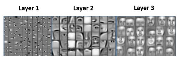
It was therefore necessary to find another approach than the classic one of ANN networks (or Multilayer Perceptron). The idea behind convolution filters is that they allow you to find patterns, shapes in images (remember the previous article which allowed you to find outlines for example). CNNs make it possible to gradually determine the different shapes and then to assemble them to find others.

The classic example is that the first layers of such a network find the basic shapes of a face: the main features, then we will detect the first shapes: nose, mouth, eyes, etc., then finally the face. and why not recognize the person, etc.

The main advantages of convolution filters are:

• The number of parameters is much smaller to find compared to an ANN type approach. In the neural network will only have to find the values of the convolution matrix (kernel) that is to say a small matrix of the type 2 × 2 or 3 × 3!
• The calculations are extremely simple because a convolution only requires multiplications and additions.

A Convolutional Neural Network (or CNN) is ultimately just a neural network that will gradually detect the characteristics of an image.

The CNN’s convolution layers

The architecture of such a network is very often articulated by a stack of convolutional layers then of deep dense layers which will do the decision work. To summarize the convolutional layers find the shapes and patterns in the image and the final layers will do the decision work (like classification for example).

Convolution layers include several filters. Each Convolution Filter – as we explained previously – the same layer will therefore extract or detect a characteristic of the image. So at the exit of a convolutional layer we have a set of characteristics which are materialized by what we call feature maps.

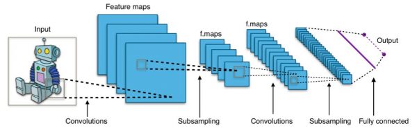
These characteristics (or resulting images of convolution filters) are then fed back into other filters, etc.

Build our own CCN now

Goal

To illustrate convolutional neural networks, we are going to create our own from scratch that will allow us to classify images. To do this we will use Python & TensorFlow 2.x (with keras) and we will use a classic dataset the MNSIT Fashion.

Dataset description

The dataset contains more than 70,000 grayscale images (see below):

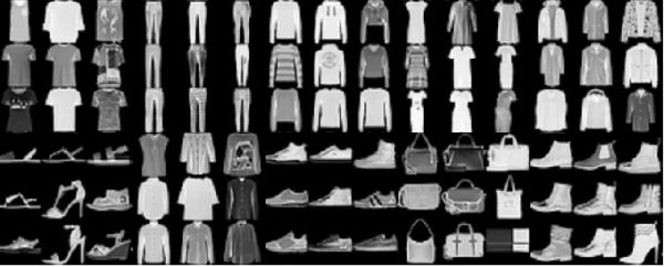
Each image is a 28 × 28 pixel square.

Good news, Tensorflow includes its images in its API so no need to bother to retrieve the dataset. To make your life easier, I suggest you use colab (the notebook will be downloadable from GitHub of course).

This data set identifies 10 types of objects (labels). These labels are coded with numbers from 0 to 9:

• 0 T-shirt/top
• 1 Trouser
• 2 Pullover
• 3 Dress
• 4 Coat
• 5 Sandal
• 6 Shirt
• 7 Sneaker
• 8 Bag
• 9 Ankle boot

Get data

Let’s start by importing the libraries:

import numpy as np
import tensorflow as tf
import matplotlib.pyplot as plt
from tensorflow.keras.layers import Dense, Conv2D, Input, Flatten, Dropout, MaxPooling2D
from tensorflow.keras.models import Model
import pandas as pd
from sklearn.metrics import classification_report,confusion_matrix
from tensorflow.keras.callbacks import EarlyStopping
import seaborn as sns

The recovery of the data set as well as the splitting is strait forward:

dataset_fashion_mnsit = tf.keras.datasets.fashion_mnist
(X_train, y_train), (X_test, y_test) = dataset_fashion_mnsit.load_data()

Now we have two datasets (training and testing). Let’s look at the distribution of labels:

pd.DataFrame(y_train)[0].value_counts()

9    6000
8    6000
7    6000
6    6000
5    6000
4    6000
3    6000
2    6000
1    6000
0    6000
Name: 0, dtype: int64

Excellent news, we have a very even distribution of these labels.

Data Preparation

Neural networks are very sensitive to data normalization. In the case of grayscale images this is very simple and since the pixels go from 0 to 255, we just have to divide all the pixels by 255:

X_train = X_train / 255
X_test = X_test / 255
print(f"Training data: {X_train.shape}, Test data: {X_test.shape}")

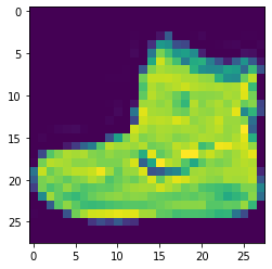
Training data: (60000, 28, 28), Test data: (10000, 28, 28)

Try to look at an image sample:

plt.imshow(X_train[0])

And its label:

y_train[0]

9

Label 9 match with an Ankle boot !

Since we have grayscale images we are missing one dimension (color: RGB). Nothing serious we will add it …

X_train = X_train.reshape(60000, 28, 28, 1)
X_test = X_test.reshape(10000, 28, 28, 1)

Modeling

I’m not going to detail everything here, but we will stack the layers of our CNN as follows:

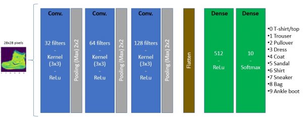
This is how to create this Neural Network with TensorFlow :

mon_cnn = tf.keras.Sequential()
 
# 3 couches de convolution, avec Nb filtres progressif 32, 64 puis 128
mon_cnn.add(Conv2D(filters=32, kernel_size=(3,3), input_shape=(28, 28, 1), activation='relu'))
mon_cnn.add(MaxPooling2D(pool_size=(2, 2)))
 
mon_cnn.add(Conv2D(filters=64, kernel_size=(3,3),input_shape=(28, 28, 1), activation='relu'))
mon_cnn.add(MaxPooling2D(pool_size=(2, 2)))
 
mon_cnn.add(Conv2D(filters=64, kernel_size=(3,3),input_shape=(28, 28, 1), activation='relu'))
mon_cnn.add(MaxPooling2D(pool_size=(2, 2)))
 
# remise à plat
mon_cnn.add(Flatten())
 
# Couche dense classique ANN
mon_cnn.add(Dense(512, activation='relu'))
 
# Couche de sortie (classes de 0 à 9)
mon_cnn.add(Dense(10, activation='softmax'))

Note: the explanation of the different hypermarameters and layers (Conv2D and pooling in particular) will come in a next article.

In order not to fumble over the number of epochs to perform, I will use the technique of EarlyStopping which allows the learning to be stopped as soon as the model begins to over-train. This allows me to neglect this parameter (epochs).

early_stop = EarlyStopping(monitor='val_loss',patience=2)

Now we can compile the model:

mon_cnn.compile(optimizer='adam',
              loss='sparse_categorical_crossentropy',
              metrics=['accuracy'])
mon_cnn.summary()

Model: "sequential_2"
_________________________________________________________________
Layer (type)                 Output Shape              Param #   
=================================================================
conv2d_2 (Conv2D)            (None, 26, 26, 32)        320       
_________________________________________________________________
max_pooling2d_2 (MaxPooling2 (None, 13, 13, 32)        0         
_________________________________________________________________
conv2d_3 (Conv2D)            (None, 11, 11, 64)        18496     
_________________________________________________________________
max_pooling2d_3 (MaxPooling2 (None, 5, 5, 64)          0         
_________________________________________________________________
conv2d_4 (Conv2D)            (None, 3, 3, 64)          36928     
_________________________________________________________________
max_pooling2d_4 (MaxPooling2 (None, 1, 1, 64)          0         
_________________________________________________________________
flatten (Flatten)            (None, 64)                0         
_________________________________________________________________
dense (Dense)                (None, 512)               33280     
_________________________________________________________________
dense_1 (Dense)              (None, 10)                5130      
=================================================================
Total params: 94,154
Trainable params: 94,154
Non-trainable params: 0

We see in the summary that our model will have to learn 94,154 parameters, so it will take a few minutes during the training phase.

Training phase (fit)

Let’s start training. Notice the number of epochs (iterations / backpropagation) of 25:

mon_cnn.fit(x=X_train, 
            y=y_train, 
            validation_data=(X_test, y_test), 
            epochs=25,
            callbacks=[early_stop])

Epoch 1/25
1875/1875 [==============================] - 59s 31ms/step - loss: 0.7872 - accuracy: 0.7077 - val_loss: 0.4386 - val_accuracy: 0.8408
Epoch 2/25
1875/1875 [==============================] - 58s 31ms/step - loss: 0.4102 - accuracy: 0.8490 - val_loss: 0.3833 - val_accuracy: 0.8625
Epoch 3/25
1875/1875 [==============================] - 58s 31ms/step - loss: 0.3345 - accuracy: 0.8752 - val_loss: 0.3404 - val_accuracy: 0.8740
Epoch 4/25
1875/1875 [==============================] - 58s 31ms/step - loss: 0.2958 - accuracy: 0.8887 - val_loss: 0.3470 - val_accuracy: 0.8747
Epoch 5/25
1875/1875 [==============================] - 58s 31ms/step - loss: 0.2694 - accuracy: 0.8987 - val_loss: 0.3225 - val_accuracy: 0.8844
Epoch 6/25
1875/1875 [==============================] - 58s 31ms/step - loss: 0.2422 - accuracy: 0.9092 - val_loss: 0.3194 - val_accuracy: 0.8862
Epoch 7/25
1875/1875 [==============================] - 57s 31ms/step - loss: 0.2329 - accuracy: 0.9115 - val_loss: 0.3220 - val_accuracy: 0.8851
Epoch 8/25
1875/1875 [==============================] - 58s 31ms/step - loss: 0.2058 - accuracy: 0.9217 - val_loss: 0.3184 - val_accuracy: 0.8898
Epoch 9/25
1875/1875 [==============================] - 58s 31ms/step - loss: 0.1969 - accuracy: 0.9271 - val_loss: 0.3080 - val_accuracy: 0.8962
Epoch 10/25
1875/1875 [==============================] - 58s 31ms/step - loss: 0.1827 - accuracy: 0.9314 - val_loss: 0.3258 - val_accuracy: 0.8890
Epoch 11/25
1875/1875 [==============================] - 58s 31ms/step - loss: 0.1740 - accuracy: 0.9318 - val_loss: 0.3455 - val_accuracy: 0.8878

Please note that the earlystopping condition allows stopping before 25 iterations (stopping after 11).

Model evaluation

TensorFlow has set aside the accuracy and loss information during the training phase and for each epoch. We just need to recover them:

losses = pd.DataFrame(mon_cnn.history.history)
losses[['accuracy', 'val_accuracy']].plot()

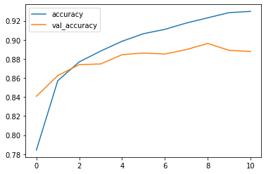
The orange curve represents the accuracy on the training data, the blue the accuracy on the test data. We also note that even if the accuracy continues to improve on the training data while the accuracyon the test data has flattened and even decreased. We then begin to over-fit, which is why the early-stopping stopped the process.

We can also see the loss curve:

losses[['loss', 'val_loss']].plot()

Let’s look at the confusion matrix (with a heat map with Seaborn):

plt.figure(figsize=(12,8))
sns.heatmap(confusion_matrix(y_test, pred),annot=True)

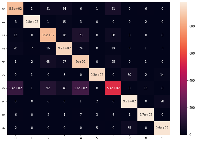
We can see that there are errors / confusion especially between shirts (6) and tops (0), which is not really surprising given the quality of the images.

Prediction

Let’s try our model on an image. For this test we will take the image from the beginning and see how our model behaves:

img = X_train[0]
mon_cnn.predict(img.reshape(1,28,28,1))

array([[3.9226734e-07, 8.9244217e-08, 6.7499624e-11, 4.7707250e-08,
        1.1513226e-08, 1.3388344e-05, 9.8523687e-09, 7.1390239e-03,
        6.6544054e-08, 9.9284691e-01]], dtype=float32)

The returned array actually offers a probability of result for each class … To get the most probable, all you have to do is take the greatest value:

np.argmax(mon_cnn.predict(img.reshape(1,28,28,1)), axis=-1)[0]

9

Our model works pretty well!

This concludes this series on image management. If you liked it, please let me know in the comments. I am well aware of having covered the subject but also had the idea somewhere … namely not to go into too much detail in order to be able to embark on this fascinating subject.