Image processing (part 1) the digital representation

In this article we will see and especially understand how images are stored in a computer just to make it usable by other softwares. In fact, this post is the first within a series that will allow us to approach image processing in general but also subsequently the place of Artificial Intelligence and especially Deep Learning in this discipline which is part of a set known as computer vision.

So let’s start our series on processing images from the beginning, which is how they are stored !

What is a digital image

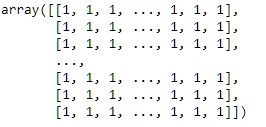
What if I tell you that an image is a matrix … will you run away? This is partially true insofar as if an image is not a matrix it is in any case how it is represented and manipulated in our digital age. Don’t worry, I’m not going to teach you an algebra lesson – at least it’s not necessary yet – but know that ultimately we represent an image as an array (or matrix) of pixels.

So what is a pixel?

Well, a pixel is quite simply a point (even if, you’ll see it looks like a square). An image is therefore a set of points organized in two dimensions (ie. matrix of dimension 2). Rather logical so far, no? Moreover, let’s take a closer look, or rather zoom in large one of your digital photos and you will see that at some point the quality of the image will deteriorate to reveal a set of small colored squares … these are our pixels!

Black and white, Grayscale and color

Actually it’s not that simple as a matrix, because if every pixel finds its logical place in a 2-dimensional matrix (just like coordinates in a map in the end), what about the color and the intensity of the pixels? So, we can distinguish 3 basic possibilities:

• The pure Black and White images
• Grayscale images
• Color images

Black & white images

This is the easiest format to understand how our images are stored.

Indeed, who says black or white says … binary ! and so 0 or 1! Indeed in the case of a black and white image the value of the pixels is a binary value (0 or 1).

Simple isn’t it ?

Grayscale images

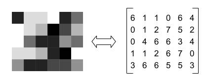
Grayscale images will of course add some nuance to the rendering. This nuance will be brought by the value of the pixels which will no longer be binary but which will evolve within a range (for example from 0 to 255). The closer the pixel value is to zero, the darker the pixel will be, and conversely the closer this value will be to 255 the brighter it will be.

The matrix which represents this type of image is therefore always a matrix of dimension 2 but with oscillating values ​​(for example between 0 and 255).

Colored images

Managing colors requires more information than managing gray levels. A color is defined by its 3 primary colors. With these three basic colors it is possible to define almost any color. In image processing, we are not talking about primary colors but rather we describe a color by the superposition of 3 channels (generally Red, Green and Blue).

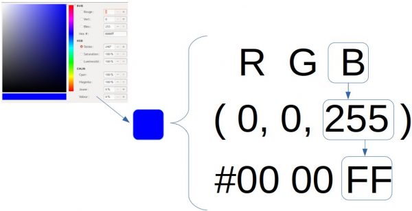
A pixel is therefore defined by a combination of red, green and blue (RGB or RGB in English). This means that for each pixel you will need an RGB tuple:

Here are some examples of colors:

• Blue (0, 0, 255)
• Red (255, 0, 0)
• Green (0, 255, 0)
• Yellow (255, 255, 0)
• White (255, 255, 255)
• Black (0, 0, 0)

Most of the time image opened by editing software or other tools (such as web / html) are defined by usingg an hexadecimal representation of these channels: for example the blue (0,0,255) becomes # 0000FF.

That being said, we must now set each pixel in the image – matrix – (remember an image is a matrix 😉 ). It’s actually like adding a new dimension:

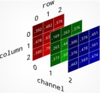
A color image is therefore represented in the form of a 3-dimensional matrix:

• Abscissa (x coordinate)
• Ordinate (y-coordinate)
• Color channel (from 0 to 2 because 3 R, G, B channels)

Note: Regarding the third dimension we can find some variations. I took the RGB model which is the most common but you can also find other modes of channel overlap (BGR in OpenCV for example, HSV / TSV, etc.). It is also possible to adjust the pixel resolution, etc.

This is the end of this first post about image processing dedicated on the images basics. In the next article we will see how the histograms will help us better analyze these images which will allow us to tackle the first retouching techniques.