Image processing (part 5) Morphologic Transformations

Part 1: The digital representation
Part 2: The histogram
Part 3: Thresholding
Part 4: Transformations
Part 5: Morphologic transformations
Part 6: Filters & convolution
Part 7: CNN

In the previous chapter of the image processing serie we saw some basic about image transformations like rotation or translations. We’re going to see in this post a different technic of transformation (called “morphological”) which can also be considered as filters. It’s an excellent transition to the next chapter, which will be dedicated to filters and more specifically to the convolution mechanism.

We’ll cover in this post the global principles of erosion and dilation of images which are widely used, especially when restoring poor quality.

Principle

The so-called “morphological transformations” are in fact based on the application of a template (or in the maths language a structuring element). We will just overlap the template on each pixel of the source image. The idea is therefore very simple, you need an image (the image to transform of course) and a single a template (which is also a matrix of course). This template can have several shapes (it can be a star, rectangle, etc.). We’ll use this shape (or template, or structuring element) as a stamp on the image we want to modify. Once this operation is done we’ll be able to make a decision of the image-template overval : if there’s only 1 values, or 0 values or both …

We can consider this operation as a transformation or as a filter. Indeed, you can find both terminologies, and finally as I said in the introduction this operation is in fact between the two concepts. Let’s see how these morphological transformations work with the two main ones: erosion and dilation. In reality there are 4 major morphological operations, namely dilation, erosion, opening and closing, in their version for grayscale images (color images are not treated here). However, as regards opening and closing, we will see that they depend on the first two, the principle of which we will detail here.

The templates (structuring elements)

To perform these transformations we need a matrix template that will actually allow us to serve as a kind of imprint on the source image. For that we will use the scikit-image library which will manage these morphological transformations effortlessly. In fact, this library already offers a certain number of templates in several shapes (star, square, etc.) as standard.

Let’s look at a very simple disc-shaped template here (good ok on 3 × 3 pixels it looks more like a cross):

import numpy as np
from skimage import data
import matplotlib as plt
from skimage import morphology
from matplotlib.pyplot import imshow, get_cmap
 
imshow(morphology.disk(1), cmap=get_cmap('gray'))

As I explained above we will apply this template to each pixel of the target image. In fact we will scan each pixel and we will look at the result of the superposition of the pixels of this template over the image.

Dilation

Let’s start with dilation (the OR for a binary image). So I find that this transformation is well named. Indeed, dilation makes it possible to enlarge an image. The height and width of this image is therefore dilated will be the sums of the heights and widths of the original image and the template. When we apply a template on the image, we will center this template on each pixel and If the pixel is equal to 1 we will make an imprint of the template on the image (centered on the pixel).

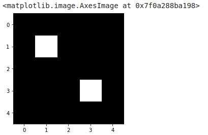
Let’s see with Python how to proceed in order to better understand the mechanism with a very simple image (with only 2 pixels at 1):

image_test = np.array([[0,0,0,0,0], 
                       [0,1,0,0,0], 
                       [0,0,0,0,0], 
                       [0,0,0,1,0], 
                       [0,0,0,0,0]])
imshow(image_test, cmap=get_cmap('gray'))

Let’s apply the dilation with the previous template with the function morphology.binary_dilation

dilation = morphology.binary_dilation(image=image_test, 
                                      selem=morphology.disk(1))
imshow(dilation, cmap=get_cmap('gray'))

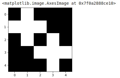
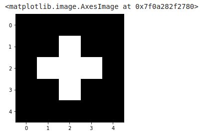
Notice in the dilated image the imprint of the two original pixels with that of the template.

We see here two crosses (corresponding to the template) which are therefore centered on the two original pixels that we had. We use dilation mainly to reconstruct shapes which has been cut.

Erosion

If you have understood the principle of dilation, erosion is no more complex … because it is quite simply the opposite (it’s the AND for a binary image). In the case of erosion, the template is placed on each pixel. Then we set the pixel to 1 if all the pixels of the placed template are 1. The result is therefore a reduction of the image.

Let’s look at another example right away:

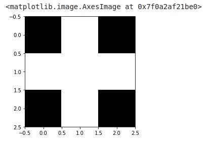
image_test = np.array([[0,0,0,0,0], 
                       [0,0,1,0,0], 
                       [0,1,1,1,0], 
                       [0,0,1,0,0], 
                       [0,0,0,0,0]])
imshow(image_test, cmap=get_cmap('gray'))

immediately perform an erosion transformation with morphology.binary_erosion

erosion = morphology.binary_erosion(image_test, morphology.disk(1))
imshow(erosion, cmap=get_cmap('gray'))

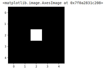
In this simple example we can clearly see that the only possibility for all the pixels of the template to be at 1 is when the same one is centered on the cross. We mainly use

Opening & closing

Without going into detail:

• The opening is the composition of the erosion by a template followed by the expansion by this same template.
• The closing is the composition of the expansion by a template followed by the erosion by this same template.

Example

Let’s take a look at what this looks like for erosion:

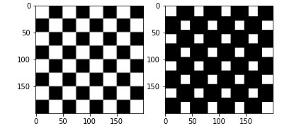
img =  data.checkerboard()
imshow(img, cmap=get_cmap('gray'))

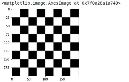
erosion = morphology.binary_erosion(img, morphology.disk(1))
imshow(img, cmap=get_cmap('gray'))

Not so obvious right ? it would actually take a magnifying glass to see the difference.

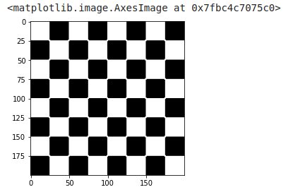
So to better see the erosion effects, we will perform this transformation several times in a row:

erosion =  data.checkerboard() 
for i in range(5):
  erosion = morphology.binary_erosion(erosion, morphology.disk(1))
imshow(erosion, cmap=get_cmap('gray'))

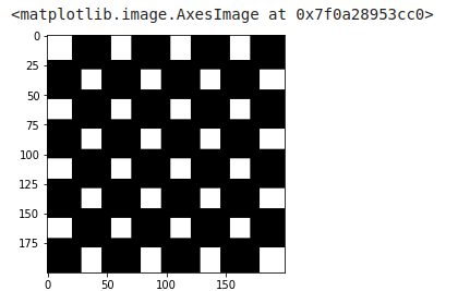
We can see much better with this result that the black pixels take up more and more space.

Here then for morphological transformations, in the next article we will discuss convolution filters and their applications.