 by
by 
Index
Why building an histogram ?
In the previous article we saw how our digital images were built and stored. This naturally brings us to the image histograms. Of course we don’t manage an image like we do for a text . Images are in fact just matrix (like a pixel map ), so we are going to manipulate them in a different and “global” way. The first line of work (and therefore retouching) is colorimetry.
We will see in this post how to analyze these color components through histograms.
Each pixel therefore being a tuple or rather a superposition of color channels (Red, Green and Blue: ie [R, G, B]). So we’ll first analyze this distribution of the three primary colors in our image.
Note: We are going to stay on images encoded in 24 bits (ie 2 to the power of 8 = 256 possible values per channel).
An image histogram is no more and no less than a graph that displays:
- On the abscissa (Val. In the graph below) the different values of channels / pixel
- On the ordinate (Nb Pixel) the number of channels / pixel that have this value
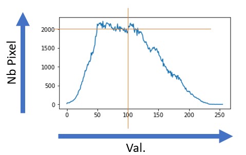
In the example graph above, we have 2000 times a pixel of value 100.
You will notice that I only put one curve in the chart. It just means that we are viewing a grayscale image, don’t panic, we’ll see that in the next paragraph.
Color, Grayscale and Black & White
How to distinguish a color image from a grayscale image from a black and white image without looking at the image? In fact, it’s pretty simple with the histograms of images:
A black and white image has a very basic (binary) histogram that only has O or 1 values (no 24-bit shades for example):
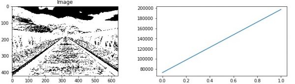
In this graph (please don’t pay attention on the line betweel 0 and 1 😉), we only have values for 0 and 1.
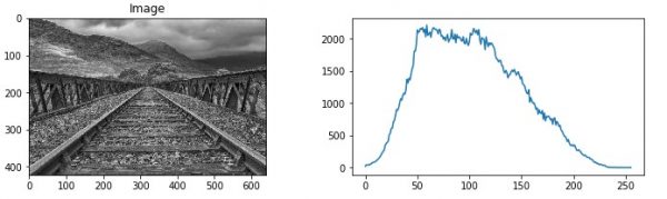
A grayscale image has only one curve (that of shades of gray):
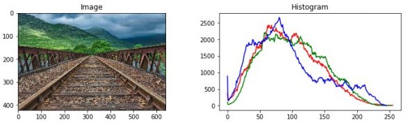
If we have a colored image we must now have the shades on the three channels (Red, Green and Blue). We therefore have 3 curves:
How to build these histograms with Python ?
With Python there are at least 3 ways to create image histograms:
- Directly using the Numpy and matplotlib library (and yes remember that our images are only matrices)
- With Scikit-Image
- Using OpenCV (Recommended because much faster)
Before starting you have to open (or even convert our images):
Read from an image file
First import the Python libraries, as follows:
import matplotlib.pyplot as plt
from skimage.io import imread, imshow
from skimage import exposure
import matplotlib.pyplot as plt
from skimage.color import rgb2gray
import numpy as np
Then just read the image with skimage’s imread () function:
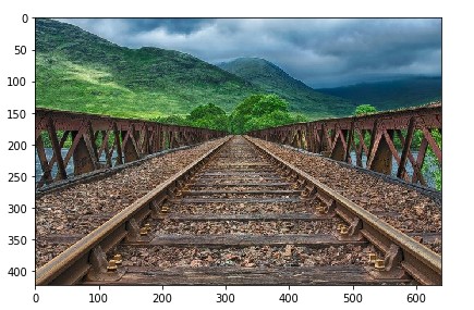
image1 = imread('railway.jpg') #, as_gray=True)
To read the image directly in grayscale (with color conversion -> grayscale) either you use the option as_gray = True as follows:
image1_Gray = imread('railway.jpg', as_gray=True)
Or you can use the rgb2gray () function after reading the color image:
image1_Gray = rgb2gray(image1)
You can display the image simply with the imshow () function:
imshow(image1)
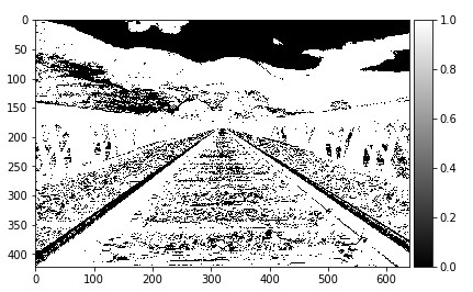
If you want to convert the image to black and white, it’s also easy. To do that, use the Numpy where method which allows you to replace the elements of an array under a condition. In the example below, I replace all elements less than 128 with 0 and all others:
im = np.where(image1_Gray>128/256, 0, 1)
imshow(im, cmap=plt.get_cmap('gray'))
Histograms with scikit-image
With scikit-image we will simply use the histogram function to plot these graphs:
def imageHist(image):
    _, axis = plt.subplots(ncols=2, figsize=(12, 3))
    if (image.ndim == 2):
        # Grascale Image
        axis[0].imshow(image, cmap=plt.get_cmap('gray'))
        axis[1].set_title('Histogram')
        axis[0].set_title('Grayscale Image')
        hist = exposure.histogram(image)
        axis[1].plot(hist[0])
    else:
        # Color image
        axis[0].imshow(image, cmap='gray')
        axis[1].set_title('Histogram')
        axis[0].set_title('Colored Image')
        rgbcolors = ['red', 'green', 'blue']
        for i, mycolor in enumerate(rgbcolors):
            axis[1].plot(exposure.histogram(image[...,i])[0], color=mycolor)
In the code above you will notice that I am looking first at the number of dimensions of the image matrix. If we have 3 dimensions, it means that we have an image with color, otherwise we are in gray level. In the case where we have an image with color we must stack the channels and therefore we will have 3 curves as follows:
Histograms with OpenCV
With OpenCV it’s just as simple and it’s also much faster in processing time. Here’s how to view the histogram of a color image:
def histogramOpenCV(_img):
    _, axis = plt.subplots(ncols=2, figsize=(12, 3))
    axis[0].imshow(_img)
    axis[1].set_title('Histogram')
    axis[0].set_title('Image')
    rgbcolors = ['red', 'green', 'blue']
    for i,col in enumerate(color):
        histr = cv.calcHist([_img],[i],None,[256],[0,256])
        axis[1].plot(histr,color = col)
In this post we have seen how to analyze an image with histograms. In the next article from the “Image Processing” series, we’ll see what these histograms are for, and we’ll use them to perform some basic image editing techniques.


6 thoughts on “Image processing (part 2) the histograms”