Image processing (part 6) Filters & Convolution

Part 1: The digital representation
Part 2: The histogram
Part 3: Thresholding
Part 4: Transformations
Part 5: Morphologic transformations
Part 6: Filters & convolution
Part 7: CNN

In the previous chapter, we saw a first kind of operations (which can also be considered as filters in a certain manner). Now we’ll generalize this principle of the small sliding window and especially to go further by adding operations on pixel values. We will therefore discuss in this article the most famous family of filters which are widely used by all editing software (such as Photoshop or Gimp). In fact, and to go further (without “sploiling” the following post either) the convolution principle will also be widely used by neural networks (Deep Learning)… but we will see that later.

Let us first focus on the principle of image filtering and more precisely of convolution.

Convolution principle

As I said in the introduction, we will keep the principle of the sliding window which will therefore run through the entire image from top to bottom and from left to right (even if in reality the order and the meaning have no importance, but it’s easier to visualize for understanding). This sliding window is called the kernel (we can clearly see the mathematical root of the concept here). There are also the terminologies of convolution kernel or just convolution mask.

Step 1

The principle is therefore very simple. We overlap the kernel on the left corner of the image matrix, as shown below. For information the kernel is the matrix with only values 0.5 in the illustration below. Then we will multiply each superimposed number and then add it all up. The result will take its place naturally as shown in the figure.

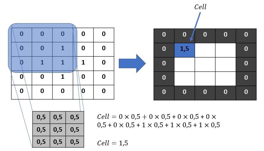
Our first pixel is therefore recalculated, we can move on to the next.

Step next …

To do this we just move the kernel one row. Then we redo the exact same operation.

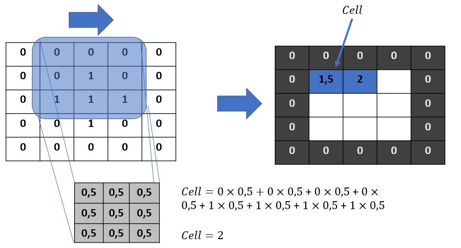
We do this of course for all the pixels of the image to be filtered. A new filtered image (matrix) should be obtained by this simple process. This process is really efficient on the one hand and very inexpensive for the machine because only additions & multiplications are carried out. We just did what is called a convolution product. This operation is moreover a bilinear, associative and commutative application.

One small detail remains! Did you notice that it was impossible to calculate the borders pixels?

Fortunately the borders rarely include large amount of pixels, and then there are few compared to the rest of the image. There are therefore several strategies to fill these borders. You can simply leave them at zero, replicate the values ​​next to them, calculate an average of the surrounding pixels, etc.

If you have understood the principle, you will now see the value of it. In fact the key to filtering is in the creation of the kernel. Fortunately, mathematicians have already worked for us by providing ready-made kernels to perform many filtering operations. We will go through a few of them.

To better familiarize yourself with this concept (if anyone is still in doubt), go to this site https://setosa.io/ev/image-kernels/ you can play with the filters and see the results directly.

Convolution with Python

We are not going to use ready-made libraries like there are. In order to illustrate the principle that we see from seeing we will directly play with matrices / pixels. We will therefore use the SciPy library for matrix convolution operations.

Let’s start by importing some libraries and add a small visualization function:

import numpy as np
from skimage import data
import matplotlib as plt
from scipy import signal
from matplotlib.pyplot import imshow, get_cmap
import matplotlib.pyplot as plt
 
def displayTwoBaWImages(img1, img2):
  _, axes = plt.subplots(ncols=2)
  axes[0].imshow(img1, cmap=plt.get_cmap('gray'))
  axes[1].imshow(img2, cmap=plt.get_cmap('gray'))

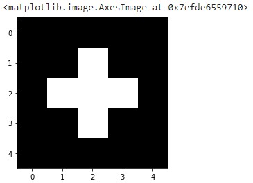
Now let’s create a very simple black and white image:

image_test = np.array([[0,0,0,0,0], 
                       [0,0,1,0,0], 
                       [0,1,1,1,0], 
                       [0,0,1,0,0], 
                       [0,0,0,0,0]])
imshow(image_test, 
       cmap=get_cmap('gray'))

Let’s create a very simple convolution kernel

kernel = np.ones((3,3), np.float32)/2

Let’s ask Scipy to make the convolution product

imgconvol = signal.convolve2d(image_test, 
                              kernel, 
                              mode='same',
                              boundary='fill', 
                              fillvalue=0)
displayTwoBaWImages(image_test, imgconvol)

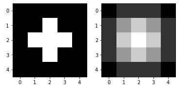
Just look at the image matrix content (try to make the calculation if you wish 😉 )

array([[0. , 0.5, 0.5, 0.5, 0. ],
       [0.5, 1.5, 2. , 1.5, 0.5],
       [0.5, 2. , 2.5, 2. , 0.5],
       [0.5, 1.5, 2. , 1.5, 0.5],
       [0. , 0.5, 0.5, 0.5, 0. ]])

This filter somehow created a blur on the base image as we can see.

Let’s see some other filters now.

Contour detection

The convolution kernel which allows to detect contours is a very simple 3 × 3 matrix:

kernel_contour = np.array([[0,1,0], 
                       [1,-4,1], 
                       [0,1,0]])

array([[ 0,  1,  0],
       [ 1, -4,  1],
       [ 0,  1,  0]])

Let’s apply the convolution filter :

imgconvol = signal.convolve2d(image, 
                              kernel_contour, 
                              boundary='symm', 
                              mode='same')
displayTwoBaWImages(image, imgconvol)
imshow(imgconvol, cmap=get_cmap('gray'))

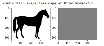
Amazing right ?

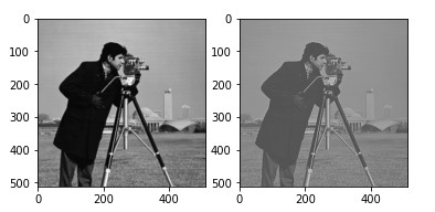
Contrast increase

The convolution kernel is now a 5 × 5 matrix:

kernel_inccontrast = np.array([[0,0,0,0,0], 
                               [0,0,-1,0,0], 
                               [0,-1,5,-1,0], 
                               [0,0,-1,0,0], 
                               [0,0,0,0,0]])

array([[ 0,  0,  0,  0,  0],
       [ 0,  0, -1,  0,  0],
       [ 0, -1,  5, -1,  0],
       [ 0,  0, -1,  0,  0],
       [ 0,  0,  0,  0,  0]])

imgcontrast = signal.convolve2d(data.camera(), 
                              kernel_inccontrast, 
                              boundary='symm', 
                              mode='same')
displayTwoBaWImages(data.camera(), imgcontrast)

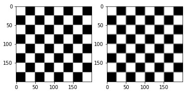
Blur

kernel = np.array([[0,0,0,0,0], 
                    [0,1,1,1,0], 
                    [0,1,1,1,0], 
                    [0,1,1,1,0], 
                    [0,0,0,0,0]])
img = signal.convolve2d(data.checkerboard(), 
                        kernel, 
                        boundary='symm', 
                        mode='same')
displayTwoBaWImages(data.checkerboard(), img)

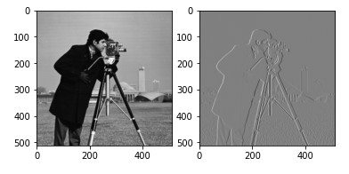
Edge reinforcement

kernel = np.array([[0,0,0], 
                   [-1,1,0,], 
                   [0,0,0,]])
img = signal.convolve2d(data.camera(), 
                        kernel, 
                        boundary='symm', 
                        mode='same')
displayTwoBaWImages(data.camera(), img)

Conclusion

There are a pretty big number of convolution kernels already provided and which allow, as we have just seen, to perform filter on the images. We will see in a future article how convolutional neural networks (CNN) will find and combine convolutional filters to detect more complex shapes.