
 by
by 
Going through the images processing serie we saw how images were structured and more importantly how to manipulate them. At the end of this serie we also set up the first concepts of convolutional neural networks in order to classify images (one of its application of course). The idea was simple: sorting images by subject. Simple at first glance … at least when the image contains only one subject. But what happens when you have several subjects in a photo? when you only want to detect a single type of subject or just locate one or more objects?
The question is immediately less obvious, isn’t it? I suggest you take a look at this subject which questioned me a lot when I got into Deep Learning, because it must be recognized that there are many articles on the net on classification but as soon as we want to go beyond this subject is immediately less prolific or much more technical.
Index
Implementing YOLO
We will see in this article, how the YOLO neural network implementation can detect several objects in a photo in one shot. The purpose of this post is not to go into the details of the implementation of this neural network (much more complex than a simple sequential CNN) but rather to show how to use the implementation which was carried out in C ++ and which is called Darknet.
You can find all the details (and the implementation itself too) of this implementation here: https://github.com/AlexeyAB/darknet
Unfortunately, as I said above the implementation of this network was done in C ++. Tha also means the binary is not portable from one platform to another. Consequently, we’ll have to recompile all of this before we can use it. But don’t worry, this task is really not tricky will be done in a single command line. We’ll see that later, don’t panic, and just trust me here 😉
Classification
We have seen it and it is indeed the first step one takes when discussing convolutional networks (CNN). Classification consists of determining what an image represents. What it represents is called a class. The list of classes is finite (categorical) and the output of the neural network will have as many neurons as there are classes. Each output has a class probability for the image that was presented as input.
I won’t stay on this topic too much, if you want more details check out this article.
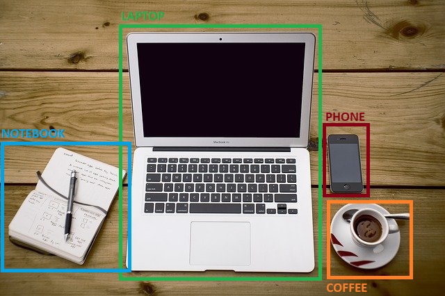
The concern with classification is that the dataset should only include data with the subject (or without of course) … otherwise it won’t do you much good. Let’s take a concrete example with the photo below.

Imagine creating a convolutional neural network (CNN) that classifies items found on a desk. Let’s assume that you have a list of classes (6 in total) like this: NOTEBOOK, LAPTOP, GLASS, DRIVE, PHONE, KEY, COFFEE, etc.
Your neural network will output something that looks something like this:
- NOTEBOOK: 97%
- LAPTOP: 98%
- GLASS: 1%
- PHONE: 85%
- DRIVE: 45%
- KEY: 9%
- COFFEE: 96%
Each percentage represents the probability that the object (or class) is in the image. This is what we now know: in this picture we have a computer, a notepad, a telephone and a coffee. But other than that (which isn’t bad actually), where are these topics?
Object detection principle
Here we are, we are delighted to see that subjects have been identified but where are they? (besides, there may be several), we now need to locate them.
Who says location, says coordinates!
In addition to finding the different class probabilities, we must therefore return a set of coordinates for each.
To detect mutiple objects in the same image, the original approach was to launch classifications by sliding smaller windows over the entire image … but this approach was long and above all required to reread the source image several times. The basic idea behind YOLO is to only do one pass (read) of the image (YOLO = You Only Look Once). Result detection is really much faster!
YOLO preparation
Let’s move on to practice … I suggest that you now use this network to detect images.
For this we will use:
- Google colab (this way we will have the same execution environment, and even better naked ones will be able to use GPUs for free).
- The most popular Darknet implementation available on Github: https://github.com/AlexeyAB/darknet
You won’t need more, a simple basic laptop will do!
Notebook creation & config
Create your notebook in Google colab, if you forgot or don’t know how to do it, look at the following article.
Once the notebook has been created, the GPUs must be activated.
For this:
- Select the menu: Execution
- Choose Change the type of execution
- Select GPU (Hardware Accelerator)
Darknet preparation
In Google colab, we must now import the darknet project, for this we can use the commands directly in the cells by prefixing them with the ! character.
!git clone https://github.com/AlexeyAB/darknet
Cloning into 'darknet'...
remote: Enumerating objects: 14997, done.
remote: Total 14997 (delta 0), reused 0 (delta 0), pack-reused 14997
Receiving objects: 100% (14997/14997), 13.38 MiB | 11.68 MiB/s, done.
Resolving deltas: 100% (10194/10194), done.
It should take some time to import all of the project content into your colab environment.
Warning: you will have to re-import the project each time you open the notebook.
To use the GPUs that are available to you via Google colab, you must now also change some darknet network configuration values. To do this you have to open the makefile and modify some entries (GPU, CUDNN, CUDNN_HALF). We will also take the opportunity to activate OpenCV and LIBSO (in order to recover the necessary libraries later).

Of course, you can edit the file directly, but when you re-open the notebook, you will have to start the manual operation again. I propose instead to automate this via the use of sed script like this (to be placed directly in the next cell of the notebook):
%cd darknet
!sed -i 's/OPENCV=0/OPENCV=1/' Makefile
!sed -i 's/GPU=0/GPU=1/' Makefile
!sed -i 's/CUDNN=0/CUDNN=1/' Makefile
!sed -i 's/CUDNN_HALF=0/CUDNN_HALF=1/' Makefile
!sed -i 's/LIBSO=0/LIBSO=1/' Makefile
Now you can compile the darknet code :
!make
mkdir -p ./obj/
mkdir -p backup
chmod +x *.sh
g++ -std=c++11 -std=c++11 -Iinclude/ -I3rdparty/stb/include -DOPENCV `pkg-config --cflags opencv4 2> /dev/null || pkg-config --cflags opencv` -DGPU -I/usr/local/cuda/include/ -DCUDNN -DCUDNN_HALF -Wall -Wfatal-errors -Wno-unused-result -Wno-unknown-pragmas -fPIC -Ofast -DOPENCV -DGPU -DCUDNN -I/usr/local/cudnn/include -DCUDNN_HALF -fPIC -c ./src/image_opencv.cpp -o obj/image_opencv.o
./src/image_opencv.cpp: In function ‘void draw_detections_cv_v3(void**, detection*, int, float, char**, image**, int, int)’:
./src/image_opencv.cpp:926:23: warning: variable ‘rgb’ set but not used [-Wunused-but-set-variable]
...
You will see that it takes a little time on the one hand and that on the other hand you will have a lot of Warning … don’t panic, that’s okay.
The network is now compiled and ready to be used, we must now recover the weights because we will of course recover a pre-trained network:
!wget https://github.com/AlexeyAB/darknet/releases/download/darknet_yolo_v3_optimal/yolov4.weights
--2021-05-04 07:26:27--  https://github.com/AlexeyAB/darknet/releases/download/darknet_yolo_v3_optimal/yolov4.weights
Resolving github.com (github.com)... 140.82.121.3
Connecting to github.com (github.com)|140.82.121.3|:443... connected.
HTTP request sent, awaiting response... 302 Found
...
Saving to: ‘yolov4.weights’

yolov4.weights      100%[===================>] 245.78M  58.5MB/s    in 6.5s

2021-05-04 07:26:33 (37.6 MB/s) - ‘yolov4.weights’ saved [257717640/257717640]
It must also take a little while depending on your connection … note that the file is rather big … it means that the YOLO network is deep! really deep as you’ll see later the number of layers implemented.
First try in command line
Our neural network is ready to use. We will now test it to see how it works. For that we will use images which are in the data directory of the network (you can as well import and test with yours).
Here is the photo we will use (dog.jpg):
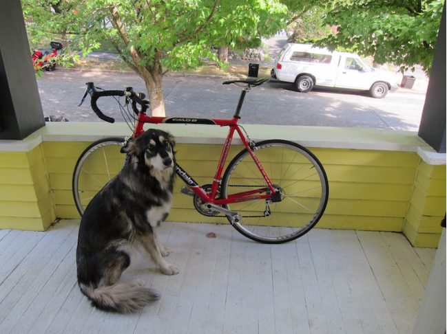
Let’s launch via the command line (in a colab cell). The syntax is fairly simple and requires the network configuration file (cfg), the weights and of course the source image:
!./darknet detector test cfg/coco.data cfg/yolov4.cfg yolov4.weights data/dog.jpg
CUDA-version: 11000 (11020), cuDNN: 7.6.5, CUDNN_HALF=1, GPU count: 1
 CUDNN_HALF=1
 OpenCV version: 3.2.0
 0 : compute_capability = 370, cudnn_half = 0, GPU: Tesla K80
net.optimized_memory = 0
mini_batch = 1, batch = 8, time_steps = 1, train = 0
   layer   filters  size/strd(dil)      input                output
   0 Create CUDA-stream - 0
 Create cudnn-handle 0
conv     32       3 x 3/ 1    608 x 608 x   3 ->  608 x 608 x  32 0.639 BF
   1 conv     64       3 x 3/ 2    608 x 608 x  32 ->  304 x 304 x  64 3.407 BF
   2 conv     64       1 x 1/ 1    304 x 304 x  64 ->  304 x 304 x  64 0.757 BF
   3 route  1 		                           ->  304 x 304 x  64
   4 conv     64       1 x 1/ 1    304 x 304 x  64 ->  304 x 304 x  64 0.757 BF
   5 conv     32       1 x 1/ 1    304 x 304 x  64 ->  304 x 304 x  32 0.379 BF
   6 conv     64       3 x 3/ 1    304 x 304 x  32 ->  304 x 304 x  64 3.407 BF
...
 160 conv    255       1 x 1/ 1     19 x  19 x1024 ->   19 x  19 x 255 0.189 BF
 161 yolo
[yolo] params: iou loss: ciou (4), iou_norm: 0.07, obj_norm: 1.00, cls_norm: 1.00, delta_norm: 1.00, scale_x_y: 1.05
nms_kind: greedynms (1), beta = 0.600000
Total BFLOPS 128.459
avg_outputs = 1068395
 Allocate additional workspace_size = 6.65 MB
Loading weights from yolov4.weights...
 seen 64, trained: 32032 K-images (500 Kilo-batches_64)
Done! Loaded 162 layers from weights-file
 Detection layer: 139 - type = 28
 Detection layer: 150 - type = 28
 Detection layer: 161 - type = 28
data/dog.jpg: Predicted in 174.085000 milli-seconds.
bicycle: 92%
dog: 98%
truck: 92%
pottedplant: 33%
Once again the trace is rather verbose, but if you look at the last lines you can find some interesting information. We find in effect the different classes (objects) which have been detected with their probability (confidence in the detection). So we have in this photo a bicycle, a dog, a truck… and a potted plant ??? Hey, that’s weird, let’s take a closer look, especially since the score is 33% (we certainly have an object that looks more or less like a potted plant in fact).
By default, the command line creates a file (predictions.jpg) with a frame for each object. We will display it via Python in colab:
import matplotlib.pyplot as plt
from skimage.io import imread, imshow

image = 'data/dog.jpg'
def display(_image):
  img1 = imread(_image)
  img2 = imread('predictions.jpg')
  fig, axes = plt.subplots(ncols=2)
  fig.set_size_inches(18.5, 10.5)
  axes[0].set_axis_off()
  axes[0].imshow(img1)
  axes[1].set_axis_off()
  axes[1].imshow(img2)
  plt.tight_layout()

display(image)
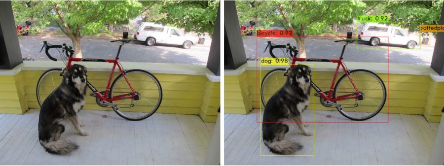
Look at the bottom right… it seems that our network has confused (at 33% which is rather not bad in fact) a trash can with a potted plant.
Our command line offers several options, here are some of them:
Adjustment of the detection threshold: Thresold [-thresh] in order to only report objects detected above a certain threshold:
!./darknet detector test cfg/coco.data cfg/yolov4.cfg yolov4.weights data/dog.jpg -thresh 0.5
Do not return the image as output via the option [-dont_show]
!./darknet detector test cfg/coco.data cfg/yolov4.cfg yolov4.weights data/person.jpg -dont_show
To return coordinates and information in text format [-ext_output]
There are many other options available on github
Using Python
We used the binary to start the detection but we can also use Python via the darknet_images.py file
!python darknet_images.py --weights yolov4.weights --input data/dog.jpg
Now if we want to use this network into a Python program there are several wrappers in pyPI. However we can also use the Python files provided by darknet:
from darknet_images import image_detection
from darknet import load_network
import cv2

weights = 'yolov4.weights'
input = 'data/dog.jpg'
datafile = './cfg/coco.data'
cfg = './cfg/yolov4.cfg'
thresh= 0.5

network, class_names, class_colors = load_network(cfg, datafile,  weights, 1)

image, detections = image_detection(
                                    input,
                                    network,
                                    class_names,
                                    class_colors,
                                    thresh
                                    )
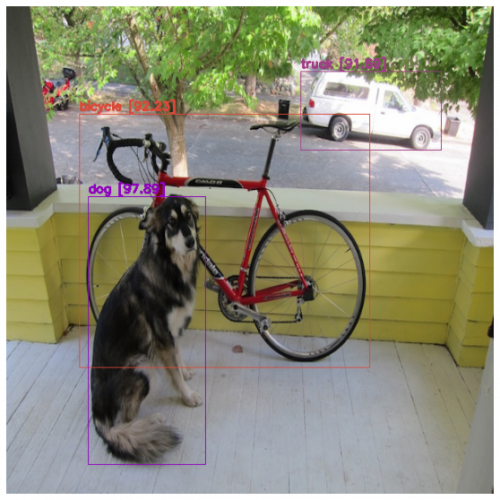
The first two lines import the prebuilt functions into darknet (in the darknet.py and darknet_images.py files), then we use these functions directly. The result is an image (matrix) and a python detection object which provides the detection information:
Let’s look at the result:
detections
[('truck',
  '91.69',
  (454.5706787109375,
   130.06553649902344,
   174.90374755859375,
   98.58089447021484)),
 ('bicycle',
  '92.23',
  (271.85552978515625,
   292.2611389160156,
   362.61639404296875,
   315.614990234375)),
 ('dog',
  '97.89',
  (174.8762969970703,
   404.4398193359375,
   146.10897827148438,
   334.0611267089844))]
We find the 3 objects detected with their probability and coordinates.
Let’s look at the picture:
fig = plt.gcf()
fig.set_size_inches(18, 10)
plt.axis("off")
plt.imshow(cv2.cvtColor(image, cv2.COLOR_BGR2RGB))
Conclusion
In this article I didn’t want to go into details about the concepts of YOLO / Darknet nor all the possibilities this YOLO implementation has to offer. The idea was to show how to simply use this network and above all to give a starting point for the use of this type of network. One thing is clear, YOLO is fast and having tested it on a lot of photos the level of confidence is really correct … now as always in neural networks there are really a lot (or even too many) ways to configure it but also adapt it to specific detections … a future article maybe ?
The sources of the notebook in my Github
Please let me your comments below


3 thoughts on “YOLO (Part 1) Introduction with Darknet”