by
by In the last article in the image processing series we discussed convolutional neural networks. We even created one, but it must be recognized that it is very simple. The problem when we want to have good results is that we need a lot of labelled images but also a lot of resources because very quickly we have to stack a good number of layers in our deep neural network in order to have great accuracy.
In short, the question of time, resources but also the choice of hyperparameters of the neural network can become key for many projects.
What if we reused a piece of existing, pre-trained neural network?
This is exactly the goal we are trying to achieve with Transfer Learning! and to do this there are a lot of neural networks that are already available. We will start in this article with one of the most famous: VGG.
Index
What is VGG ?
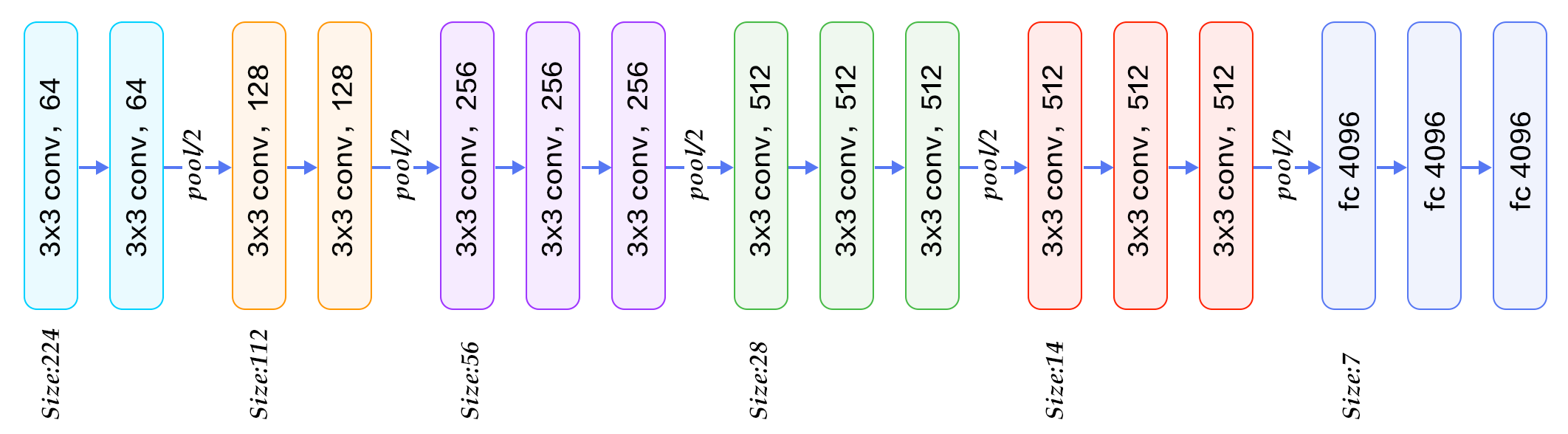
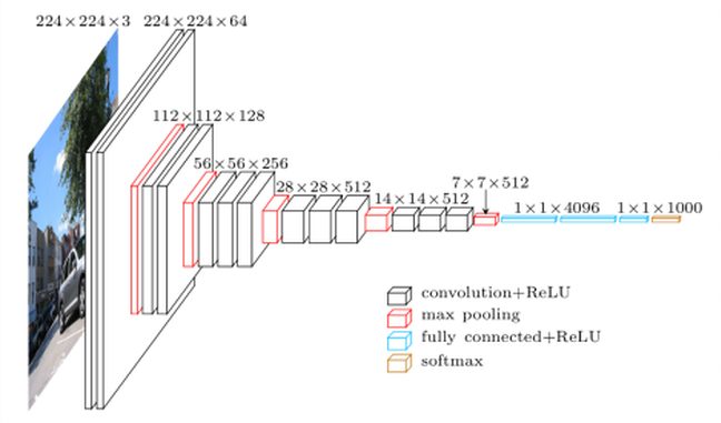
VGG16 is a convolutional neural network model designed by K. Simonyan and A. Zisserman. The implementation details can be found in the document “Very Deep Convolutional Networks for Large-Scale Image Recognition”. This model achieves 92.7% test accuracy in ImageNet, which aggregates more than 14 million images belonging to 1000 classes. Why vgg-16 and good simply because this neural network includes 16 deep layers:
So of course, you could create this neural network by yourself – and from scratch – then find out the best hyperparameters to finally train it. But that would take a lot of your time and resources… so why not use all the settings in this model and see how to complete this network by adding custom layers to it?
This is exactly what we are going to do in this article, and we will doing it with some labels/classes that VGG has not ever been trained for. Crazy isn’t it? that’s kind of the magic of convolutional neural networks. We will in fact be able to reuse the feature map mechanisms that were produced by the VGG but to detect new shapes.
VGG & TensorFlow
Good news, Tensorflow provides the VGG-16 model as standard and therefore makes Transfer Learning very easy.
In fact it provides as standard other pre-trained models such as:
- VGG16
- VGG19
- ResNet50
- Inception V3
- Xception
You will see that the reuse of these models is child’s game 🙂
Let’s build a fruit detector!
To test our custom VGG-16 Transfer Learning model we will use a dataset made up of fruit images (131 types of fruit to be exact). You can find this dataset on Kaggle at the following address: https://www.kaggle.com/moltean/fruits
Be careful if you want to follow me step by step and create your own neural network, know that you will need power (GPU / TPU). So I suggest you do like me and create a notebook in Kaggle.
You can watch mine here: https://www.kaggle.com/shiftbc/fruit-and-vgg
Dataset presentation & discovery
The dataset is structured by directory (and you will see that this structure has not been done randomly):
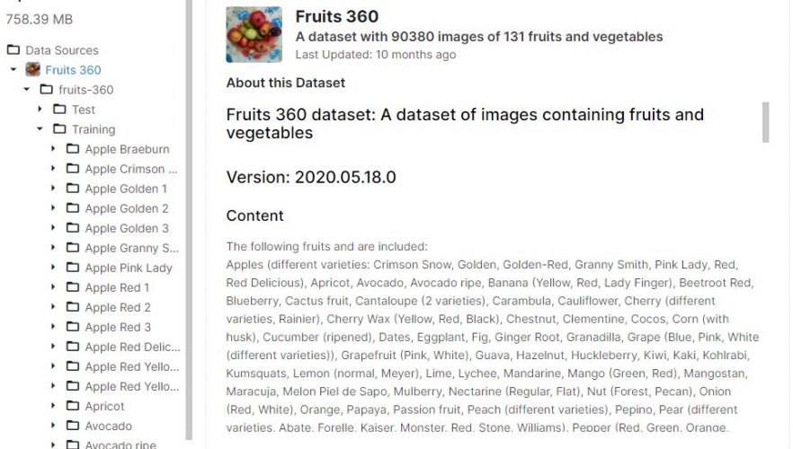
We have two datasets: Training and Test. In each of these directories there are sub-directories (labels) in which we have photos of the different fruits.
Here is some additional information that may be useful later:
- Images: 90483
- One fruit per image
- Training: 67703 images
- Test: 19543 images
- Labels/fruits: 131
- Image Size: 100×100 pixels
First steps …
Commençons par importer les librairies nécessaires :
import numpy as np
import pandas as pd
from glob import glob

from keras.layers import Input, Lambda, Dense, Flatten
from keras.models import Model
from keras.applications.vgg16 import VGG16
from keras.applications.vgg16 import preprocess_input
from keras.preprocessing import image
from keras.preprocessing.image import ImageDataGenerator
from tensorflow.keras.callbacks import EarlyStopping

import numpy as np
import matplotlib.pyplot as plt
from skimage.io import imread, imshow
Let’s look at an image :
image = imread("/content/drive/MyDrive/Colab Notebooks/fruits-360/Training/Apple Braeburn/0_100.jpg")
plt.imshow(image)
Perfect we have a beautiful apple in color (RGB).
image.shape
(100, 100, 3)The size of the images is confirmed 100 by 100 pixels.
Data Augmentation with TensorfFlow
90,483 images is fine, but much more would be even better. I will use this article to introduce what is called “data augmentation”. The principle is very simple, the idea is to decline an image by shifting, rotating, zooming in order to duplicate it in several copies. From an image we can therefore have x new images and therefore improve the learning of our model by this method.
With TensorFlow we will use what are called Generators. there are several, but here we are going to use the ImageDataGenerator () Image Generator which will do all this duplication work for us and automatically.
To start, we configure the way we will create the image combinations with the ImageDataGenerator () function
Then we will use and apply this Generator to our two datasets (Training and Test)
src_path_train = "/content/drive/MyDrive/Colab Notebooks/fruits-360/Training"
src_path_test = "/content/drive/MyDrive/Colab Notebooks/fruits-360/Test"
batch_size = 32

image_gen = ImageDataGenerator(
        rescale=1 / 255.0,
        rotation_range=20,
        zoom_range=0.05,
        width_shift_range=0.05,
        height_shift_range=0.05,
        shear_range=0.05,
        horizontal_flip=True,
        fill_mode="nearest",
        validation_split=0.20)

# create generators
train_generator = image_gen.flow_from_directory(
  src_path_train,
  target_size=IMSIZE,
  shuffle=True,
  batch_size=batch_size,
)

test_generator = image_gen.flow_from_directory(
  src_path_test,
  target_size=IMSIZE,
  shuffle=True,
  batch_size=batch_size,
)
Found 67703 images belonging to 131 classes.
Found 19543 images belonging to 131 classes.
Here it is! simple isn’t it?
Modeling
We will now create the model from VGG-16.
3 minimum things to remember here:
- We use the VGG16 class provided by TensorFlow (here we use imagenet weights), include_top specifies that we take the whole model except the last layer
- We tag the layers of the neural network so as not to overwrite the learning already retrieved (layer.trainable = False)
- We add a new Dense layer at the end (we could add others by the way), it is this layer that will make the choice of this or that fruit.
NBCLASSES = 131
train_image_files = glob(src_path_train + '/*/*.jp*g')
test_image_files = glob(src_path_test + '/*/*.jp*g')

def create_model():
    vgg = VGG16(input_shape=IMSIZE + [3], weights='imagenet', include_top=False)

    # Freeze existing VGG already trained weights
    for layer in vgg.layers:
        layer.trainable = False

    # get the VGG output
    out = vgg.output

    # Add new dense layer at the end
    x = Flatten()(out)
    x = Dense(NBCLASSES, activation='softmax')(x)

    model = Model(inputs=vgg.input, outputs=x)

    model.compile(loss="binary_crossentropy",
                  optimizer="adam",
                  metrics=['accuracy'])

    model.summary()

    return model

mymodel = create_model()
Model: "model_1"
_________________________________________________________________
Layer (type)                 Output Shape              Param #
=================================================================
input_2 (InputLayer)         [(None, 100, 100, 3)]     0
_________________________________________________________________
block1_conv1 (Conv2D)        (None, 100, 100, 64)      1792
_________________________________________________________________
block1_conv2 (Conv2D)        (None, 100, 100, 64)      36928
_________________________________________________________________
block1_pool (MaxPooling2D)   (None, 50, 50, 64)        0
_________________________________________________________________
block2_conv1 (Conv2D)        (None, 50, 50, 128)       73856
_________________________________________________________________
block2_conv2 (Conv2D)        (None, 50, 50, 128)       147584
_________________________________________________________________
block2_pool (MaxPooling2D)   (None, 25, 25, 128)       0
_________________________________________________________________
block3_conv1 (Conv2D)        (None, 25, 25, 256)       295168
_________________________________________________________________
block3_conv2 (Conv2D)        (None, 25, 25, 256)       590080
_________________________________________________________________
block3_conv3 (Conv2D)        (None, 25, 25, 256)       590080
_________________________________________________________________
block3_pool (MaxPooling2D)   (None, 12, 12, 256)       0
_________________________________________________________________
block4_conv1 (Conv2D)        (None, 12, 12, 512)       1180160
_________________________________________________________________
block4_conv2 (Conv2D)        (None, 12, 12, 512)       2359808
_________________________________________________________________
block4_conv3 (Conv2D)        (None, 12, 12, 512)       2359808
_________________________________________________________________
block4_pool (MaxPooling2D)   (None, 6, 6, 512)         0
_________________________________________________________________
block5_conv1 (Conv2D)        (None, 6, 6, 512)         2359808
_________________________________________________________________
block5_conv2 (Conv2D)        (None, 6, 6, 512)         2359808
_________________________________________________________________
block5_conv3 (Conv2D)        (None, 6, 6, 512)         2359808
_________________________________________________________________
block5_pool (MaxPooling2D)   (None, 3, 3, 512)         0
_________________________________________________________________
flatten_1 (Flatten)          (None, 4608)              0
_________________________________________________________________
dense_1 (Dense)              (None, 131)               603779
=================================================================
Total params: 15,318,467
Trainable params: 603,779
Non-trainable params: 14,714,688
_________________________________________________________________
We find all the layers of VGG-16 upstream and the added layer (Dense / 131) at the end. Also note the number of pre-trained parameters (14,714,688) that will be reused.
Model Training
The training will take a long time, but then a long time if you don’t have a GPU locally, use colab or kaggle if you don’t have one.
epochs = 30
early_stop = EarlyStopping(monitor='val_loss',patience=2)

mymodel.fit(
  train_generator,
  validation_data=test_generator,
  epochs=epochs,
  steps_per_epoch=len(train_image_files) // batch_size,
  validation_steps=len(test_image_files) // batch_size,
  callbacks=[early_stop]
)
Epoch 1/10
2115/2115 [==============================] - 647s 304ms/step - loss: 0.0269 - accuracy: 0.6334 - val_loss: 0.0085 - val_accuracy: 0.8802
Epoch 2/10
2115/2115 [==============================] - 289s 136ms/step - loss: 0.0037 - accuracy: 0.9787 - val_loss: 0.0055 - val_accuracy: 0.9295
Epoch 3/10
2115/2115 [==============================] - 290s 137ms/step - loss: 0.0018 - accuracy: 0.9923 - val_loss: 0.0047 - val_accuracy: 0.9391
Epoch 4/10
2115/2115 [==============================] - 296s 140ms/step - loss: 0.0012 - accuracy: 0.9959 - val_loss: 0.0043 - val_accuracy: 0.9522
Epoch 5/10
2115/2115 [==============================] - 298s 141ms/step - loss: 8.8540e-04 - accuracy: 0.9967 - val_loss: 0.0040 - val_accuracy: 0.9524
Epoch 6/10
2115/2115 [==============================] - 298s 141ms/step - loss: 6.6982e-04 - accuracy: 0.9985 - val_loss: 0.0037 - val_accuracy: 0.9600
Epoch 7/10
2115/2115 [==============================] - 299s 142ms/step - loss: 5.5506e-04 - accuracy: 0.9984 - val_loss: 0.0035 - val_accuracy: 0.9613
Epoch 8/10
2115/2115 [==============================] - 353s 167ms/step - loss: 4.5906e-04 - accuracy: 0.9988 - val_loss: 0.0037 - val_accuracy: 0.9599
Epoch 9/10
2115/2115 [==============================] - 295s 139ms/step - loss: 3.9744e-04 - accuracy: 0.9987 - val_loss: 0.0033 - val_accuracy: 0.9680
Epoch 10/10
2115/2115 [==============================] - 296s 140ms/step - loss: 3.4436e-04 - accuracy: 0.9993 - val_loss: 0.0035 - val_accuracy: 0.9671
Quick evaluation
score = mymodel.evaluate_generator(test_generator)
print('Test loss:', score[0])
print('Test accuracy:', score[1])
Test loss: 0.003505550790578127
Test accuracy: 0.9680007100105286
With an accuracy of 97% we can say that the model did its job very well… and did you see? in so few lines of Python / Tensorflow.
Once again I invite you to look at my notebook on Kaggle: https://www.kaggle.com/shiftbc/fruit-and-vgg
Try adding layers, changing settings, etc.