 by
by 
In this article (which is the 3rd post of the image processing series) we will see how to use the image histograms we saw in the post 2 so as to do some basic editing. We are therefore going to analyze and from the histograms and change the intensity values of the different color channels of our image. This technique is called thresholding, and is very often used as an image preprocessing in order to be able to do other operations afterwards (like shape detection, etc.). We will use, like in previous articles Python language to manipulate images
Index
Grayscale image thresholding
Lest’s first import the needed Python libraries :
import matplotlib.pyplot as plt
from skimage.io import imread, imshow
from skimage import exposure
import matplotlib.pyplot as plt
from skimage.color import rgb2gray
import numpy as np
from skimage.filters import threshold_mean, threshold_otsu
import pandas as pd

image1_Gray = imread('railway.jpg', as_gray=True)
We can now open the image (initially in color) as grayscale.
Let’s display its histogram (Cf. post 2) :
def histGrayScale(img, _xlim=255, _ylim=2400):
    _, axes = plt.subplots(ncols=2, figsize=(12, 3))
    ax = axes.ravel()
    ax[0].imshow(img, cmap=plt.get_cmap('gray'))
    ax[0].set_title('Image')
    hist = exposure.histogram(img)
    ax[1].plot(hist[0])
    # to provide a better display we just change the plot display
    ax[1].set_xlim([0, _xlim])
    ax[1].set_ylim([0, _ylim])
histGrayScale(image1_Gray)
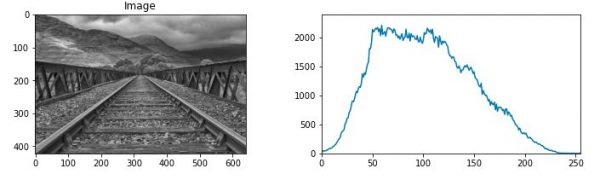
In this grayscale image we see that the majority of pixels have an intensity of 50 to 120.
Let’s force all the pixels above 120 to 255 to see what happens. In Python this is a very simple (Numpy) operation:
im = np.where(image1_Gray>120/256, 1, image1_Gray)
histGrayScale(im, 254, 2400)
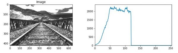
The result is quite visible, the image getting closer and closer to pure black and white. Also notice the histogram which is naturally cut off from 120 (the right part no longer exists at all).
You can also remove the left part of the histogram (pixels less than 50):
im = np.where(im<50/256, 0, im)
histGrayScale(im, 254, 2400)
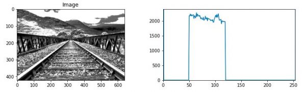
See the result and the differences in details :
Get the images statistics
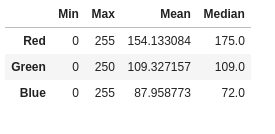
We have seen the importance of the data presented by our histograms for performing thresholds. Histograms provide a comprehensive understanding of the image, but how do we determine our thresholds? (like those of 120 and 50 that we used previously). Some statistical data like the mean, the median and even why not the quartiles could be useful. Here is a little Python function that shows us these elements:
def RGBStats(image):
    colors = []
    for i in range(0, 3):
        max_color =np.max(image[:,:,i])
        min_color =np.min(image[:,:,i])
        mean_color = np.mean(image[:,:,i])
        median_color = np.median(image[:,:,i])
        row = (min_color, max_color, mean_color, median_color)
        colors.append(row)
    return pd.DataFrame(colors,
                        index = ['Red', ' Green', 'Blue'],
                        columns = ['Min', 'Max', 'Mean', 'Median'])

RGBStats(image1)
Binary image thresholding based on the mean
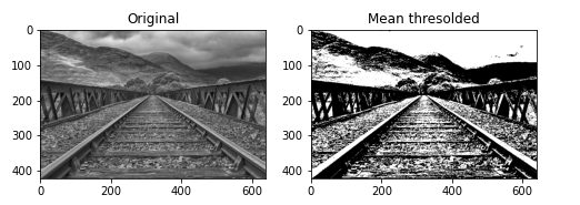
Very often the thresholding technique is used to create a black and white image: this is called binary thresholding. In these cases it seems logical to base it on the average of the pixels. Anything below the average will be set to 0 and anything above 1. The skimage threshold_mean () function does it all by itself for you:
def thresholdMeanDisplay(image):
thresh = threshold_mean(image)
binary = image > thresh
fig, axes = plt.subplots(ncols=2, figsize=(8, 3))
ax = axes.ravel()
ax[0].imshow(image, cmap=plt.cm.gray)
ax[0].set_title('Original')
ax[1].imshow(binary, cmap=plt.cm.gray)
ax[1].set_title('Mean thresolded')
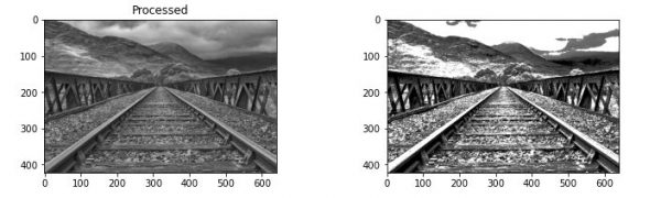
thresholdMeanDisplay(image1_Gray)
Otsu Thresholding
Otsu thresholding is a threshold calculation technique based on the shape of the histogram of the image. We will use the ready-made skimage threshold_otsu () function.
def thresholdOtsuDisplay(image):
    thresh = threshold_otsu(image)
    binary = image > thresh
    fig, axes = plt.subplots(ncols=2, figsize=(8, 3))
    ax = axes.ravel()
    ax[0].imshow(image, cmap=plt.cm.gray)
    ax[0].set_title('Original')
    ax[1].imshow(binary, cmap=plt.cm.gray)
    ax[1].set_title('Otsu thresolded')

thresholdOtsuDisplay(image1_Gray)
Colored image thresholding
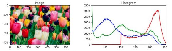
For color images, the thresholding principle is the same but with the difference that we will do this operation by channels (RGB).
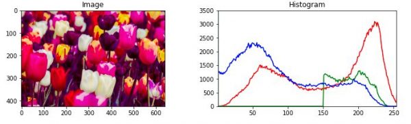
Let’s take a color image, and look at its histogram:
image1 = imread('tulip.jpg')
def histColor(img):
    _, axes = plt.subplots(ncols=2, figsize=(12, 3))
    axes[0].imshow(img)
    axes[0].set_title('Image')
    axes[1].set_title('Histogram')
    axes[1].plot(exposure.histogram(img[...,0])[0], color='red')
    axes[1].plot(exposure.histogram(img[...,1])[0], color='green')
    axes[1].plot(exposure.histogram(img[...,2])[0], color='blue')
    axes[1].set_xlim([1, 254])
    axes[1].set_ylim([0, 3500])
histColor(image1)
Just display the three channels separately :
rgb = ['Reds','Greens','Blues']
_, axes = plt.subplots(1, 3, figsize=(15,5), sharey = True)
for i in range(3):
   axes[i].imshow(image1[:,:,i], cmap = rgb[i])
   axes[i].set_title(rgb_list[i], fontsize = 15)
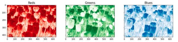
You will notice the “negative vision” … take a closer look at the 4 tulips at the bottom center… they are white and therefore appear logically dark on all 3 channels (white being the sum of all colors).
Let’s do a thresholding on the green channel by removing the low intensity greens until 150:
thresold_G = 150
image1_modified = image1.copy()
image1_modified[:,:,1] = np.where(image1[:,:,1]>thresold_G,
                                  image1[:,:,1],
                                  0)
histColor(image1_modified)
This is the result of the image that has removed a good part of its green channel.

6 thoughts on “Image processing (part 3) Image Thresholding”