Sentiment analysis on movie reviews

The objective of this article is to show through a concrete and French case the method to perform a sentiment analysis with Python.

Purpose of the use case

For this article we will analyze movie reviews in French. Since it is not easy to find datasets of this type (in French I mean), I suggest that you go and look for data directly from their source, on allociné for example.

Here are the steps that we will go through together:

• Data recovery
• Data preparation (normally this phase is of course preceded by a profiling phase but we will spend it to go faster).
• Preparation of the model and datasets (training & testing)
• Modelization
• Result

Here are the big steps we are going to take, so let’s go!

The problem to be addressed

As I told you, we will retrieve the data directly from the Allociné site. In other words we are going to scrape the pages that interest us on this site, namely the reviews of people for the films Inception and Bigfoot .

Note: Review pages have the same structure, so it will be the same job regardless of the movie.

If you go to the reviews page you will see that only two types of information are of interest to us: the viewer’s rating and their comment.

Why the note? because we are going to train a supervised type model and therefore the note will help us in this classification.

We are therefore indeed in a classification problem. We could of course try to give the score according to the comment but in order to start simple we will reduce the problem to a binary classification. To put it simply, reading the commentary, was the viewer satisfied or not? for this we will consider that a score above 3 is considered satisfactory. Below the opinion is negative.

• Note> 3: Positive feedback
• Rating <= 3 Negative opinion

Let’s scrape the spectactor opinion data

We only have to “scrape” two areas (in red below):

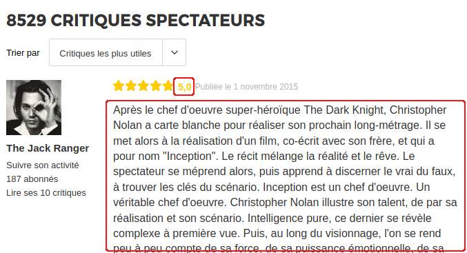
These two areas are tagged in HTML with the tags:

• Note: ‘// span [@ class = “stareval-note”]’
• Description: ‘// div [@ class = “content-txt review-card-content”]’

The method for scraping this page is described in the following article . Here is the result :

import requests
import lxml.html as lh
import pandas as pd

url = 'http://www.allocine.fr/film/fichefilm-143692/critiques/spectateurs/'
uri_pages = '?page='
nbPages = 400
tags = ['//span[@class="stareval-note"]', \
        '//div[@class="content-txt review-card-content"]' ]
cols = ['Note', 'Description' ]

page = requests.get(url)
doc = lh.fromstring(page.content)

def getPage(url):
    page = requests.get(url)
    doc = lh.fromstring(page.content)

    # Get the Web data via XPath
    content = []
    for i in range(len(tags)):
        content.append(doc.xpath(tags[i]))

    # Gather the data into a Pandas DataFrame array
    df_liste = []
    for j in range(len(tags)):
        tmp = pd.DataFrame([content[j][i].text_content().strip() for i in range(len(content[i]))], columns=[cols[j]])
        tmp['key'] = tmp.index
        df_liste.append(tmp)

    # Build the unique Dataframe with one tag (xpath) content per column
    liste = df_liste[0]
    for j in range(len(tags)-1):
        liste = liste.join(df_liste[j+1], on='key', how='left', lsuffix='_l', rsuffix='_r')
        liste['key'] = liste.index
        del liste['key_l']
        del liste['key_r']
    
    return liste

def getPages(_nbPages, _url):
    liste_finale = pd.DataFrame()
    for i in range (_nbPages):
        liste = getPage(_url + uri_pages + str(i+1))
        liste_finale = pd.concat([liste_finale, liste], ignore_index=True)
    return liste_finale

liste_totale = getPages(nbPages, url)
liste_totale.to_csv('../../datasources/films/allocine_inception_avis.csv', index=False, quoting=csv.QUOTE_NONNUMERIC)

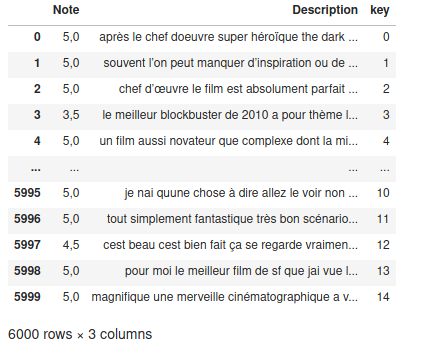
It is enough to reproduce this code (by changing of course the URL and the number of pages) to the desired films and the turn and played. Normally you should now have at least two viewer notice files that will look like this:

Data preparation

Now that we have our datasets, we will have to prepare them in order to be able to model our sentiment analysis.

For this we will use several techniques:

• Regular expressions to remove noise (punctuation, etc.) from comments.
• From NLP to tokeniser and reduce the body of each comment (for example to keep only the important words via stopwords)
• Of bags of words to “transform” our words into numbers which can then be operated in a machine learning algorithm such as a logistic regression example.

Note: for more details on these techniques do not hesitate to refer to the articles which refer to them (Cf. links above).

Remove noises from comments

For this we will use regular expressions and remove the punctuation elements but also the carriage returns and other characters useless for our analysis.

<pre class="wp-block-syntaxhighlighter-code">REMPLACE_SANS_ESPACE = re.compile("[;:!\'?,\"()\[\]]")
REMPLACE_AVEC_ESPACE = re.compile("(<br\s*/><br\s*/>)|(\-)|(\/)|[.]")
PUR_NOMBRE = re.compile("[0-9]")
 
def setClassBin(i):
    if (float(i.replace(',', '.')) > 3):
        return 1
    else:
        return 0
     
def preprocess(txt):
    txt = [PUR_NOMBRE.sub("", (str(line)).lower()) for line in txt] # retire les nombres (comme les années)
    txt = [line.replace('\n', ' ')  for line in txt] # Retire les \n (retours chariots)
    txt = [REMPLACE_SANS_ESPACE.sub("", line.lower()) for line in txt]
    txt = [REMPLACE_AVEC_ESPACE.sub(" ", line) for line in txt]
    return txt</pre>

Simplification of comment data

To start we will use the stopwords that we saw when we discussed NLP ( SpaCy and NLTK ):

X['Description'] = pd.DataFrame(preprocess(X['Description']))
french_stopwords = set(stopwords.words('french'))
filtre_stopfr =  lambda text: [token for token in text if token.lower() not in french_stopwords]
X['Description'] = [' '.join(filtre_stopfr(word_tokenize(item))) for item in X['Description']]

Once the stopwords have been initialized in French, we create a function that will filter the comments with this list (made up of the “tokenized” comment in words).

Here is our comments are now filtered to their essentials.

Preparation of labels

There is not much to do here, but remember that we are getting grades 1 to 5 and not a binary class. So we need to convert our notes:

def setClassBin(i):
    if (float(i.replace(',', '.')) > 3):
        return 1
    else:
        return 0 

yList = [setClassBin(x) for x in X.Note]
y = pd.DataFrame(yList)
X = X.drop('Note', axis=1)

Note: Let’s not forget at the end to remove the rating from the feature set.

Let’s finalize our datasets

Our data is almost ready, except that we haven’t yet converted our comments to numbers and we haven’t mixed our datasets yet. Let’s first create our datasets and concatenate our Bigfoot and Inception data:

Xtrain, ytrain = prepare_dataset(train)
Xtest, ytest = prepare_dataset(test)
Xf = pd.concat([Xtrain, Xtest])
yf = pd.concat([ytrain, ytest])

Then we will vectorize our words (word bag technic ):

from sklearn.feature_extraction.text import CountVectorizer
cv = CountVectorizer(binary=True)
cv.fit(Xf["Description"])

Xf_onehot = cv.transform(Xf["Description"])
Xtest_onehot = cv.transform(Xtest["Description"])
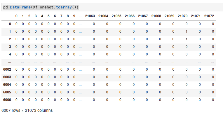
pd.DataFrame(Xf_onehot.toarray())

You should now have a nice matrix with a lot of columns (which corresponds to the number of words in the corpus):

Model training

Our data is ready, for this first exercise we are going to use a Logistic Regression algorithm .

Our first step is to find the best c hypermarameter for this algorithm. We will try a few to see the best:

X_train, X_val, y_train, y_val = train_test_split(Xf_onehot, yf, train_size = 0.75)

for c in [0.01, 0.05, 0.25, 0.5, 1]:
    lr = LogisticRegression(C=c)
    lr.fit(X_train, y_train)
    print ("Précision pour C=%s: %s" % (c, accuracy_score(y_val, lr.predict(X_val))))

Précision pour C=0.01: 0.8468708388814914
Précision pour C=0.05: 0.8901464713715047
Précision pour C=0.25: 0.9027962716378163
Précision pour C=0.5: 0.9014647137150466
Précision pour C=1: 0.8981358189081226

It seems that the best value of c is 0.25 in our case.

Let’s train the model now, and look at its accuracy against the known labels:

final_model = LogisticRegression(C=0.25)
final_model.fit(Xf_onehot, yf)
print ("Précision: %s" % accuracy_score(ytest, final_model.predict(Xtest_onehot)))

Précision: 0.8571428571428571

Without great optimizations we have a small 85 %.

The complete sources (Notebook Jupyter) are in the Github datacorner.fr in the texts \ sentiment-analysis directory.

Conclusion

The objective of this article was to show an example of an implementation from A to Z of a sentiment analysis algorithm. Without much effort we got a score of 85%, which is not too bad. Of course we could change or optimize the algorithm (use a Bayes algorithm or an SVM for example), but it is especially in the work on the corpus that we could considerably improve the performance of our model. It is a painstaking job of course and constant adjustments that make this type of problem quite complex to maintain until you have enough training data.