 by
by Index
Introduction
Why the logistic regression? well without doubt because this algorithm is one of the most used in Data Sciences. In fact, some regression algorithms can also be used for classification (and vice versa of course). Logistic regression (or logit) is often used to estimate the probability that an observation belongs to a particular class (the typical example is spam detection).
To summarize it is a binary classifier.
The principle is simple, if the estimated probability is greater than 50%, then the model predicts that the observation belongs to this class (called the positive class, with label “1”), otherwise, it predicts that it belongs to the other class (the negative class, with label “0”). here it reminds us somewhere of how analog to digital conversions work
Implementation
First of all we need a dataset! I suggest starting with the classic titanic dataset (to download from the Kaggle site ). This dataset includes the list of passengers (survivors or not: label) with a certain number of characteristics (gender, ticket price, etc.). It’s perfect to start. Our objective ? simple, from this dataset, predict if a passenger with certain characteristics (the same as the dataset of course) would have had a chance to survive this disaster!
Kaggle.com makes our life easier and offers two datasets: one to train our model and another to test it ( train.csv and test.csv ).
We will use the Python toolkit: Scikit-learn ( sklearn.linear_model.LogisticRegression)
Data observation
First of all we will observe the data.
import pandas as pd
titanic = pd.read_csv("./data/train.csv")
titanic.head(5)
Then it is interesting to use the Pandas functions in order to take a closer look at the data.
Use the functions for this:
titanic.info()
titanic.describe(include='all')
titanic.PassengerId.describe(include='all')
Here’s what the main columns store here:
| PassengerId | Passenger ID (unique) |
| SisbSp | (Sibling and Spouse): the number of family members of the passenger of the same generation |
| Parch | (Parent and Child): the number of family members of the passenger of different generation |
| Fare | The price of the ticket |
| Survived (Etiquette / Label) | Survivor (1) or not (0) |
Cross-validation with logistic regression
First, let’s prepare the model (ie. The feature matrix X as well as the label matrix y). The Python function returns these two matrices with only 3 characteristics (Cf. above):
def Prepare_Modele_1(X):
    target = X.Survived
    X = X[['Fare', 'SibSp', 'Parch']]
    return X, target
X, y = Prepare_Modele_1(titanic.copy())
In order to refine our analysis we are going to run cross validations on our training game of logistic regression algorithms (here we will run 5 cross validations which will randomly take 4/5 of the overall game and test on the remaining 1/5) :
from sklearn.model_selection import cross_val_score
def myscore(clf, X, y):
    xval = cross_val_score(clf, X, y, cv = 5)
    return xval.mean() *100
This gives a good idea of the reliability of our algorithm. This is particularly relevant since our dataset is small!
For a first effortless test we obtain an honorable 67.45%
Let’s try a first prediction …
We can also directly test / run the logistic regression algorithm. First of all, we train the model with the function fit ():
lr2 = LogisticRegression()
lr2.fit(X, y)
Then we ask for predictions. to do this, we must of course give the predict () function the same typology of vector as the one used to train it (roughly the same characteristics):
lr2.predict([[5.1,1,0]])
lr2.predict([[100.1,1,0]])
You will notice that the price of the ticket seems to have a real impact on the odds of survival.
Out of curiosity, look at the scoring of your model:
lr2.score(X, y)
Here I have a score of 68.12%
We will see in a future article how to improve our model by adjusting the training characteristics.
The Jupyter notebook from this first part is available here .
Let’s refine our model by adding new features
Characteristic Class
For that just view it with a graph:
import numpy as np
import matplotlib.pyplot as plt

def plt_feature(feature, bins = 30):
    m = titanic[titanic.Survived == 0][feature].dropna()
    s = titanic[titanic.Survived == 1][feature].dropna()
    plt.hist([m, s], label=['Morts', 'Survivants'], bins = bins)
    plt.legend(loc = 'upper left')
    plt.title('Distribution relative de %s' %feature)
    plt.show()
plt_feature('Pclass')
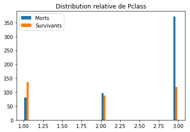
We immediately notice that the notion of class has a link with survival (people in class 3 had a much higher probability of death than those in class 1, for example). It is therefore a characteristic to be taken into account. So let’s prepare our new matrix of characteristics and try a new logistic regression
def Prepare_Modele_2(X):
    target = X.Survived
    to_del = ['Name', 'Age', 'Cabin', 'Embarked', 'Survived', 'Ticket', 'Sex']
    for col in to_del : del X[col]
    return X, target
X, y = Prepare_Modele_2(titanic)
myscore(lr1, X, y)
We obtain a score of 67.9% … In short, disappointing, but ultimately rather logical, because our model already took into account the price of the ticket which is most certainly a link with the class (a 1st class ticket is necessarily more expensive!) .
Characteristic Gender
Let’s look at the sex distribution histograms:
parSexe = [1 if passager == 'male' else 0 for passager in titanic.Sex]
titanic["SexCode"] = [1 if passager == 'male' else 0 for passager in titanic.Sex]
m = titanic[titanic.Survived == 0]["SexCode"].dropna()
s = titanic[titanic.Survived == 1]["SexCode"].dropna()
plt.hist([m, s], label=['Morts', 'Survivants'], bins = 30)
plt.legend()
Note: Unfortunately we cannot use character type categorical variables. To remedy this we will use Python’s magical Lists comprehensions to add a new column to our list: [1 if passager == 'male' else 0 for passager in titanic.Sex]
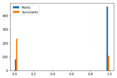
There seems to be a link between sex and survival (would “women and children first” have been appropriate that night?). Perfect we will add this variable to our existing model:
def Prepare_Modele_3_Test(X):
    target = X.Survived
    to_del = ['Name', 'Age', 'Cabin', 'Embarked', 'Survived', 'Ticket']
    for col in to_del : del X[col]
    return X, target
X, y = Prepare_Modele_3_Test(titanic.copy())
X.head(5)
myscore(lr1, X, y)
And here is the drama ! a nice Python error returned stating that it cannot convert Sex to Float.ValueError: could not convert string to float: 'male'
This is normal because the algorithm only knows how to work with digital data, so you have to transform the sex into digital data (binary here) for it to work:
def Prepare_Modele_3(X):
    target = X.Survived
    sexe = pd.get_dummies(X['Sex'], prefix='sex')
    X = X.join(sexe)
    to_del = ['Name', 'Age', 'Cabin', 'Embarked', 'Survived', 'Ticket', 'Sex']
    for col in to_del : del X[col]
    return X, target
X, y = Prepare_Modele_3(titanic)
myscore(lr1, X, y)
And this is rather a good surprise because our score jumps 10 positions to reach 79.4%
Weighting of characteristics / variables
It can be interesting to see the weighting of the characteristics (ie the importance that the algorithm gives them), for that it is enough to display the attribute of LogisticRegression () as follows:
lr1.fit(X, y)
lr1.coef_
(Be careful, the weighting is only calculated after a call to fit (), if you don’t make this call you will get an error!)
Here is the result : array([[ 1.20981540e-04, -7.76272690e-01, -2.48122601e-01, -8.67013029e-02, 4.01693066e-03, 1.85813513e+00, -8.29102327e-01]])
Each element of the vector below indicates the weight of the model variable (a positive value increases the probability a negative decreases it).
Note: We can add other variables to refine even more obviously: play on age for example and more generally on the quality of the data (missing values, etc.).
Conclusion
We have seen in this article how logistic regression can help us determine (classify) a binary diagnosis. This algorithm is also widely used in medicine. We have also noticed that before changing the algorithm or method, it was first essential to refine the characteristics (addition, modification, etc.): this is feature engineering. Finally, adding related characteristics had only little impact on the result (we will see that this is all the more true, even compulsory in the case of algorithms like Naives Bayes).
The Jupyter notebook from this second part is available on Github.