The Stochastic Gradient Descent (SGD) & Learning Rate

When I finished my last article about gradient descent, I realized that there were two important points missing. The first concerns the stochastic approach (SGD) when we have too large data sets, the second being to see very concretely what happens when we choose the wrong value of the learning rate. I will therefore take advantage of this article to finally continue the previous article 😉

Why Stochastic ?

If we refer to Wikipedia:

Stochastic refers to the property of being well described by a random probability distribution. Although stochasticity and randomness are distinct in that the former refers to a modeling approach and the latter refers to phenomena itself, these two terms are often used synonymously. Furthermore, in probability theory, the formal concept of a stochastic process is also referred to as a random process.

Wikipedia

Ok, but why are we talking about process / random choice here?

Remember in the article on Gradient Descent, at some point in the algorithm we have to sum all the values in the dataset in order to evaluate the gradient:

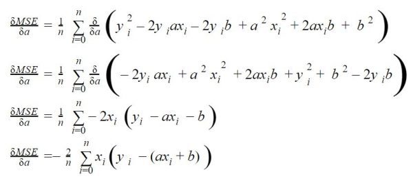
In this example, no worries as we had a very little dataset. Just now imagine that you have thousands or even millions of data! it is clear that performing this calculation at each iteration (epochs) will become very costly in terms of time and machine resources.

So instead of taking all the data, why not work on samples every epochs? We will just have to choose these samples at random …

This is exactly what a stochastic gradient descent (or SGD) offers. This is a gradient descent but will focus on different samples of the overall dataset at each iteration.

What consequences?

Nothing is free or ideal in real life, and such an approach also has consequences that we will see together. Since the gradient is calculated on the basis of random samples, we must keep in mind 2 things in order to maintain a certain accuracy in our algorithm:

• The sample size (or mini batch) is important and must be adjusted correctly. We call this parameter the batch_size. Too small it is not representative of the dataset in the iteration (epochs) and too large, well it is no interest!
• The number of epochs should naturally increase. In fact, given that the batch data (samples) are chosen randomly, we must be sure to cover all the data in order to once again be representative.

To summarize, with the SGD we have an additional hyper-parameter to adjust : the batch_size.

Let’s see what’s that look like in Python ?

The code is basically the same as the one we put in place in the article on gradient descent. We are just going to add the notion of batch size and of course the random selection of data (mini batch).

We will also just add some data:

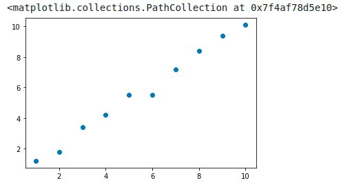
X = [1.0, 2.0, 3.0, 4.0, 5.0, 6.0, 7.0, 8.0, 9.0, 10.0]
y = [1.2, 1.8, 3.4, 4.2, 5.5, 5.5, 7.2, 8.4, 9.4, 10.1]
plt.scatter(X,y)

For the random selection of data in an array we will use the np.random.randint function (below). This method randomly selects numbers (in the example below) 3 numbers. These randomly drawn numbers are then used as indexes from which we will retrieve the data for the global dataset with the Numpy take() method.

# Select randomly 3 items index (random from 0 to length)) in the dataset
idx = np.random.randint(0, len(X), 3)
# take the items by selecting their index
np.take(X, idx)

array([4., 1., 1.])

Here we have just chosen at random 3 points in the data set. Let’s generalize this mechanism within our gradient descent function :

def SGD(_X, _y, _learningrate=0.06, _epochs=5, _batch_size=1):
    a, b = 0.2, 0.5
    trace = pd.DataFrame(columns=['a', 'b', 'mse'])
 
    for i in range(_epochs):
        # stochastic stuff / create batch (data packages) here
        indexes = np.random.randint(0, len(_X), _batch_size) # random sample
        X = np.take(np.array(_X), indexes)
        y = np.take(np.array(_y), indexes)
 
        N = len(X)
        delta = y - (a*X + b)
         
        # Updating a and b
        a = a - _learningrate * (-2 * X.dot(delta).sum() / N)
        b = b - _learningrate * (-2 * delta.sum() / N)
 
        trace = trace.append(pd.DataFrame(data=[[a, b, mean_squared_error(np.array(y), a*np.array(X)+b)]], 
                                          columns=['a', 'b', 'mse'], 
                                          index=['epoch ' + str(i+1)]))
 
    return a, b, trace

The notion of batch size is implemented in lines 7, 8 and 9. Also notice the addition of the _batch_size parameter which allows you to configure the size of the mini-batches.

First try

Let’s try our function with the same hyper-parameters that we used previously (see article) with a batch size of 5 (i.e. half the data set)

a, b, trace = SGD(X, y, _epochs=10, _batch_size=5,  _learningrate=0.06)
displayResult(a, b, trace, X, y)

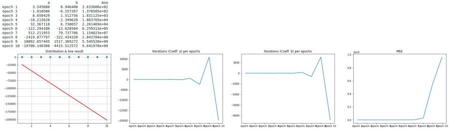
Ouch!

We can see that in the first graph the line (directed by the coefficients a and b) is totally false (note the values of a and b after 10 epochs). But above all what should put the tip in the ear is the cost curve (4th graph). The cost literally explodes from the 7th iteration.

Clearly our gradient descent comes down to a descent to hell!

The learning rate choice

This example actually illustrates an extreme case that can occur when the Learning rate is too high. During the gradient descent, between two steps we then skip the minimum and even sometimes we can completely diverge from the result to arrive at something totally wrong. The diagram below (particularly the 3rd image) illustrates this case:

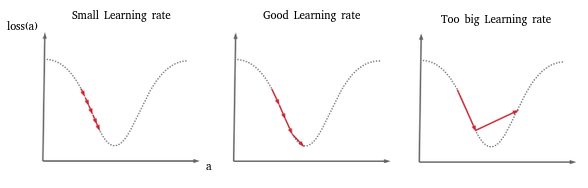
We therefore chose a too big learning rate.

Second chance

We will greatly reduce this learning rate to see what it gives and to verify our theory (we will go from 0.06 to 0.0005)

a, b, trace = SGD(X, y, _epochs=10, _batch_size=5,  _learningrate=0.0005)
displayResult(a, b, trace, X, y)

This is much better, but we can clearly see on the first graph that the line is still far from being the right one (we can easily guess the right line which should be more inclined). In addition, the cost curve (the 4th) still oscillates too much, which means that our gradient descent makes a yoyo between the two ends of the dish. Nevertheless, we can clearly see that the trend is good.

And the last try …

The trend is good, now it may be enough to just let the system continue to approach the minimum. So we’re just going to increase the number of iterations and go to 100 epochs.

a, b, trace = SGD(X, y, _epochs=100, _batch_size=5,  _learningrate=0.0005)
displayResult(a, b, trace, X, y)

Awesome ! the line generally follows the points well (1st graph), and we can clearly see that the cost has reached a minimum and above all remains stable (the curve crashes to never go up again). I think we can say that we have found our parameters a and b!

Conclusion

In this article we saw how to optimize the gradient descent when we had large datasets (by using mini-batches) with the SGD. Of course, this adds a new hyper parameter (batch size), but when we are dealing with models with several parameters and millions of data, this option will no longer be an option.

We then saw the disastrous consequences of a poor choice of the hyper-parameter learning rate. By playing on this hyper parameter but also with the number of iterations (epochs) we saw how we could adjust our gradient descent.

These adjustments are fundamental when creating a model. The idea of these articles was of course to show you in a very simplistic way how they work and especially how to “play” with them. The sources are also available on Github. Do not hesitate to make your own experiences.