The Gradient Descent

How to talk about Machine Learning or even Deep Learning without addressing the – famous – gradient descent? There are many articles on this subject of course, but most of the time you have to read several of these ones so as to fully understand all the mechanisms behind the scene. Sometimes too mathematical or not enough! I will try here to explain how it works simply and step by step in order to try to demystify the subject (big deal is’t it ?)

Promise not too much math … but a few, sorry!

If the math formulas are really too bloated for you, no worries, they are only there to explain the overall mechanism of gradient descent. You can therefore pass them quickly … I would say that what should be remembered from this article is: The iterative principle of gradient descent but also and above all the associated vocabulary (epochs, learning rate, MSE, etc.) because you will find them as hyperparameters in many Machine / Deep Learning algorithms.

What is Gradient Descent?

To explain what gradient descent is, you must understand why and where this idea comes from. I really like the image of the man at the top of a mountain who is got lost and must find his village below. But the terrain is steep, there are lots of trees, etc. In short, how to get home? Of course he can try and try again by this direction or the other one, but honestly, it’s not very efficient!

Instead, why not step up to the lowest surface around him? then start again like this for each step.

In fact it’s like selecting the direction which is quite simply given to it by the slope of the ground and in a progressive way.

This is exactly the principle of Gradient Descent. The idea is to solve a mathematical equation but not in a “traditional” way, but by putting in place an algorithm that will move step by step to approach the the most the solution. Why ? and quite simply because it is the only way to solve certain equations which are not unsolvable as they are ! And this will be the case when you have many features to manage in your model.

An equation ? but what is he talking about?

Yes, I did say the annoying word: equation. Let’s just look at an equation as a rule that governs behavior or observations. For example, imagine we measure the filling of a container every minute for 3 minutes. This consequently gives us 3 points, for each point we have on the abscissa (x) the minute, and on the ordinate (y) the volume poured.

Here are the 3 points:

• A (1, 1.2)
• B (2, 1.8)
• C (3, 3.4)

Obviously there is no straight line (which goes through these three points):

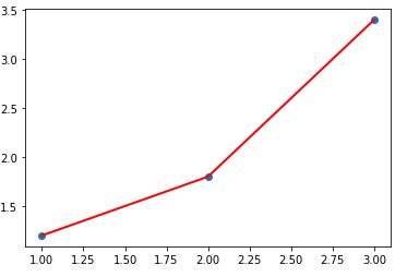
With these conditions, it is difficult to know the volume that will be fill in minute 4, 5, etc. We just know that the law is a quite linear rule, or at least it approximates. So let’s try to find this law in order to find out the following values. In fact, this is called a Linear Regression. But here, we will experiment the gradient descent mechanism which will allow us to find our famous rule.

The objective is therefore to find out the parameters a and b of the equation on the right:

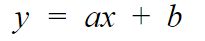
Once we have this line equation, it will be extremely easy to find out the values for all minutes like 5, 6, etc. But how to do it ? certainly not by chance! Don’t forget also we have in our case a very simple case (with only 1 feature) but sometimes there can be several hundred (and more) of these features. So we definitely have to find a sucure way to figure out the solution. Remember the man at the top of the mountain, we’ll do the same approach.

The cost function

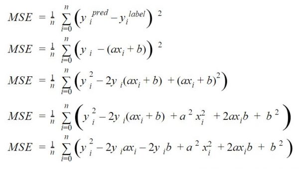
The cost function is the key as it measures the error between the estimatation we made and the known label (we are in a supervised mode). Let’s say we are going to take it step by step and with each step we take we are going to see if we are far from what we expected: this is the error rate. In our case we will use the MSE cost function (mean squared error) which has the advantage of strongly penalizing big errors:

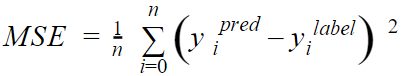
This function calculates the difference (squared, hence the high penalty mentioned above) of each result compared to the expected label. The values xi and yi are the values of the points (observations) that we have already noted.

Let’s just replace the values with the right equation we expect (y = ax + b), and we get:

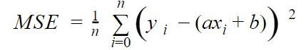
This cost function can also be represented by a parabola (squared function).

Find the line closest to the points is also find the minimum of this cost function.

In fact, the cost function measures the sum of the distances between each point observed and the line assumed to be the best. In the diagram below, we measure this distance by the squared sum of the lines in green (e1, e2 and e3 because we have 3 observations):

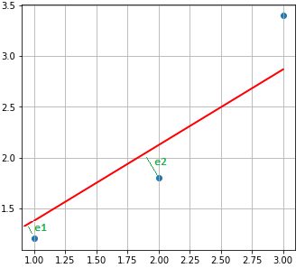
The result must therefore be as small as possible.

Cost function variation (considering a & b variables)

If your high school math class isn’t too far off, you need to remember:

• A parabola has only one minimum (good news)
• We measure the slope of a curve with a derivative
• We can derive a function / several variables (partial derivatives)

Note: Our case is so simple that we would be tempted to say that our function reaches its minimum when its derivative is zero … but once again we are in a very (too) simple case which has only two variables. In reality it would not be possible to proceed in this way.

Let’s develop our previous equality on the cost function step by step:

Now let’s look at its derivatives according to the two variables that interest us: a and b

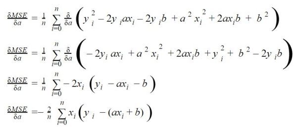
Derivative according to a

By deriving according to a we look at the variations of the cost curve according to the values of a (it is a parabola, remember). To find out parameter a we must therefore find the minimum of this derivative function.

Take a look at it step by step:

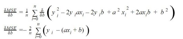
Derivative according to b

We also look for the value of b, we derive the same equation according to b this time:

Algorithm

We have the two (derived) functions of which we are going to find the smallest value (for a and b). For that we are going to walk these curves (one and the other) and step by step like our man at the top of his mountain.

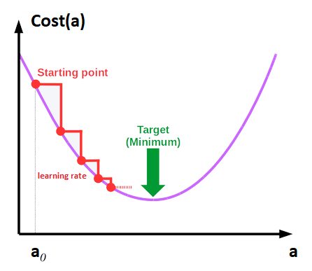
Each step (epoch) is guided by the learning rate which is in a way the length of the step. We therefore have to take several steps until we find our minimum (see stairs in red in the figure below).

In other words, the idea is therefore, step by step (or rather epoch after epoch) to approach the minimum with respect to the derivatives of our cost functions that we saw in the previous chapter:

2 comments here:

• We have to start from somewhere, so we will initialize with random values a (a0) and b (b0)
• Be careful not to choose a learning rate that is too low, otherwise you will take a long time to reach the minimum, or too high at the risk of missing it!

From scratch with Python now !

This is how that looks like using python to implement the gradient descent:

# 3 Observations
X = [1.0, 2.0, 3.0]
y = [1.2, 1.8, 3.4]
 
def gradient_descent(_X, _y, _learningrate=0.06, _epochs=5):
    trace = pd.DataFrame(columns=['a', 'b', 'mse'])
    X = np.array(_X)
    y = np.array(_y)
    a, b = 0.2, 0.5 # Random init for a and b
    iter_a, iter_b, mse = [], [], []
    N = len(X) 
     
    for i in range(_epochs):
        delta = y - (a*X + b)
         
        # Updating a and b
        a = a -_learningrate * (-2 * X.dot(delta).sum() / N) # a step for a 
        b = b -_learningrate * (-2 * delta.sum() / N) # idem for b
 
        trace = trace.append(pd.DataFrame(data=[[a, b, mean_squared_error(y, (a*X + b))]], 
                                          columns=['a', 'b', 'mse'], 
                                          index=['epoch ' + str(i+1)]))
 
    return a, b, trace

Notice in line 13 the loop which translates the steps (epochs). As for lines 17 and 18 are the Python translations of the derivatives of the cost function that we have seen in the previous chapters.

The function returns the values of a and b calculated but also a DataFrame with the values which were calculated as the epochs. Note also that for the effective calculation of the root mean square error I used the one provided by sklearn: mean_squared_error ()

Finally, a small Python function allows you to plot the results:

def displayResult(_a, _b, _trace):
  plt.figure( figsize=(30,5))
 
  plt.subplot(1, 4, 1)
  plt.grid(True)
  plt.title("Distribution & line result")
  plt.scatter(X,y)
  plt.plot([X[0], X[2]], [_a * X[0] + _b, _a * X[2] + _b], 'r-', lw=2)
 
  plt.subplot(1, 4, 2)
  plt.title("Iterations (Coeff. a) per epochs")
  plt.plot(_trace['a'])
 
  plt.subplot(1, 4, 3)
  plt.title("Iterations (Coeff. b) per epochs")
  plt.plot(_trace['b'])
 
  plt.subplot(1, 4, 4)
  plt.title("MSE")
  plt.plot(_trace['mse'])
 
  print (_trace)

Let’s try with 10 epochs now :

a, b, trace = gradient_descent(X, y, _epoch=10)
displayResult(a, b, trace)

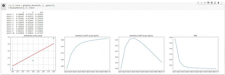
On the first graph we find the line (in red) that has just been found (with parameters a and b).

The second graph shows the different values of a found by epochs.

The third graph suggests the same for b.

The last graph shows us the evolution of the cost function per epochs. Good news, this cost decreases steadily until it reaches a minimum (close to zero). We can see that this minimum is reached quite quickly in reality (from the 2nd and 3rd epochs).

Conclusion

Let us recall the main steps of this algorithm:

• Determine the cost function
• Derive the cost function according to the parameters to find (here a and b)
• Iterate (step by step / epochs – Learning rate) to find the minimum of these derivatives

Obviously this gradient descent function in Python is not intended to be reused as is. The idea was to show what this gradient descent process looked like in a very simple case of linear regression. You can also retrieve the code (Jupyter Notebook) which was used here and why not change the hyperparameters (Learning rate and epochs) to see what is happening.