Linear Regression

Regression

Impossible to approach Data sciences or Machine Learning without going through the Linear Regression box. Of course, there are several types of regression. We saw in a previous article how to use logistic regression to perform a classification ! do you think that sounds strange? didn’t I tell you that the algorithms are divided into several families ? Regressions and classifications among others? In fact, it’s true… and then not quite! it is indeed quite possible to use and mix the algorithms.

DataScience is really cooking!

In fact, the World of Machine Learning is a world made up of uncertainties and learning. If the data that we process have their uncertainties, it seems that the, or rather the toolboxes necessary for their processing are no exception. These are mainly composed of algorithms. These algorithms mix probabilities, statistics as well as linear algebra. To be honest, it’s a very heterogeneous world, and the objective of this article is to present the simplest of supervised tools: linear regression.

Principle of Linear Regression

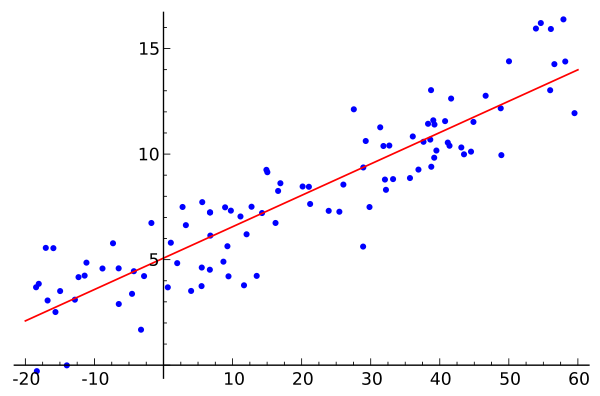
The principle is quite simple. You notice a phenomenon and incredible you detect that there is a link between the parameters of your observations (the characteristics) and the result (the label). Like any good scientist, you therefore use geometry and place your findings (blue dots) on a graph. On the x-axis you will therefore put your characteristic (we start simple with 1 only) and on the y-axis your result (label).

Incredible… your points seem, but not exactly to draw a line (therefore linear)! apart from a few uncertainties it would therefore seem that there is a linear link between your characteristic. You understood ?

Linear Regression consists in guessing which is the linear equation which links characteristic (s) and label!

To put it simply, the algorithm will try to guess what is the equation ( y = a X + b) (Cf. red line above).

Yes but how ?

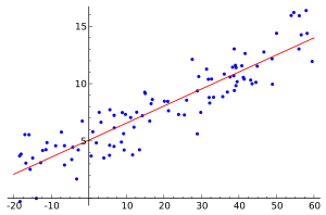
You have noticed ? there are really a lot of points, and unless you increase the thickness of the line, there are really a lot of potential candidates for our beautiful right. Which candidate to choose and how? Quite simply by taking into account the notion of error compared to the training data. Let me explain: in the learning phase we collected the necessary data (our blue points). We also have a candidate equation calculated by our algorithm… now we just have to confront it with reality.

To calculate the error rate, we can base ourselves on the distance between the real result and the calculated result (see graph above). Nothing will then prevent penalizing such and such ranges of values ​​according to dispersion factors for example. Very simply we will be able to say (on the training data) if our line responds to 80, 90 or 99%

This error rate is our cockpit to refine the parameters (a and b here).

Linear Regression with Scikit-Learn

You understand the principle … a little practice now with the Python Scikit-Learn module. To illustrate my statements above, I will start again from the Coursera training dataset ( univariate_linear_regression_dataset.csv ). This data simply represents two columns with numeric data.

Using a simple (dot) graph let’s see what this looks like (below).

import pandas as pd
import matplotlib.pyplot as plt
data = pd.read_csv('./data/univariate_linear_regression_dataset.csv')
plt.scatter (data.col2, data.col1)
plt.grid()

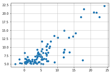
Can you imagine the right emerging? not so simple is not it but one imagines it not so badly however. let’s use the Scikit-learn library to calculate the linear regression on these data:

from sklearn import linear_model
X = data.col2.values.reshape(-1, 1)
y = data.col1.values.reshape(-1, 1)
regr = linear_model.LinearRegression()
regr.fit(X, y)
regr.predict(30)

Let’s even make a prediction with the value 30 to see the result. We get a value of 22.37, which isn’t really inconsistent, is it given the data?
Now in order to better understand what I explained to you above, I suggest you add 30 new values ​​that we will add to our learning game. for each new value we will of course make a prediction.

predictions = range(30,51)
results = []
for pr in predictions :
    results.append([pr, regr.predict(pr)[0][0]])
myResult = pd.DataFrame(results, columns=['col1', 'col2'])
myResult.head(5)

You see it now, this famous right (top right) looming? there she is ;

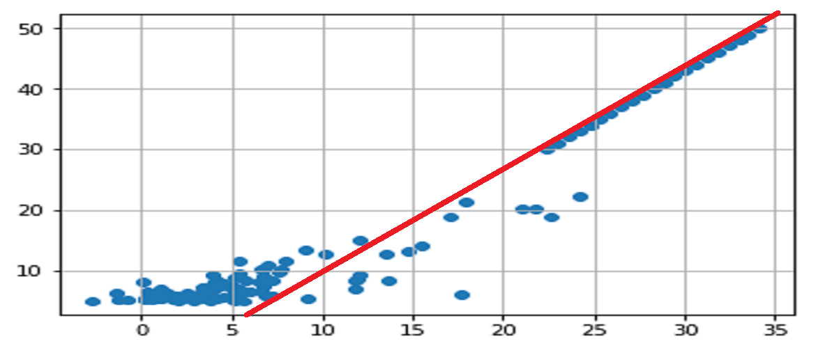
You have found that this line was not so easy to find visually and you are right because the calculation of the error rate (here very bad = 70% ) will reflect this complexity of finding a linear relationship between our two values.