Feature Scaling

What’s this again ?

My god, what is Feature Scaling? a new barbaric Anglicism (sorry as i’m french 😉 )? a new marketing side effect? Or is there something really relevant behind it? To be honest, Feature Scaling is a necessary or even essential step in upgrading the characteristics of our Machine Learning model. Why ? quite simply because behind each algorithm are hidden mathematical formulas. And these mathematical formulas do not appreciate the variations in scale of values ​​between each characteristic. And this is especially true with regard to gradient descent!

If you do nothing you will observe slowness in learning and reduced performance.

Let’s take an example. Imagine that you are working on modeling around real estate data. You will have characteristics of the type: price, surface, number of rooms, etc. Of course, the value scales of these data are totally different depending on the characteristics. However, you will have to process them using the same algorithm. This is where the bottom hurts! your algorithm will indeed have to mix prices of [0… 100,000] €, surfaces of [0… 300] m2, numbers of rooms ranging from [1 .. 10] rooms. Scaling therefore consists of bringing this data to the same level.

Fortunately Scikit-Learn will once again chew up our work, but before using this or that technique we must understand how each one works.

Preparation of tests

First of all, we will create random data sets as well as some graph functions that will help us better understand the effects of the different techniques used (above).

Here is the Python code:

import pandas as pd
import numpy as np
from sklearn.preprocessing import MinMaxScaler
from sklearn.preprocessing import StandardScaler
from sklearn.preprocessing import RobustScaler
from sklearn.preprocessing import MaxAbsScaler
import matplotlib
import matplotlib.pyplot as plt
import seaborn as sns

def plotDistribGraph(pdf):
    fig, a = plt.subplots(ncols=1, figsize=(16, 5))
    a.set_title("Distributions")
    for col in pdf.columns:
        sns.kdeplot(pdf[col], ax=a)
    plt.show()

def plotGraph(pdf, pscaled_df):
    fig, (a, b) = plt.subplots(ncols=2, figsize=(16, 5))
    a.set_title("Avant mise à l'echelle")
    for col in pdf.columns:
        sns.kdeplot(pdf[col], ax=a)
    b.set_title("Apres mise à l'echelle")
    for col in pdf.columns:
        sns.kdeplot(pscaled_df[col], ax=b)
    plt.show()

def plotGraphAll(pdf, pscaled1, pscaled2, pscaled3):
    fig, (a, b, c, d) = plt.subplots(ncols=4, figsize=(16, 5))
    a.set_title("Avant mise à l'echelle")
    for col in pdf.columns:
        sns.kdeplot(pdf[col], ax=a)
    b.set_title("RobustScaler")
    for col in pscaled1.columns:
        sns.kdeplot(pscaled1[col], ax=b)
    c.set_title("MinMaxScaler")
    for col in pscaled2.columns:
        sns.kdeplot(pscaled2[col], ax=c)
    d.set_title("StandardScaler")
    for col in pscaled3.columns:
        sns.kdeplot(pscaled3[col], ax=d)
    plt.show()

np.random.seed(1)
NBROWS = 5000
df = pd.DataFrame({
    'A': np.random.normal(0, 2, NBROWS),
    'B': np.random.normal(5, 3, NBROWS),
    'C': np.random.normal(-5, 5, NBROWS),
    'D': np.random.chisquare(8, NBROWS),
    'E': np.random.beta(8, 2, NBROWS) * 40,
    'F': np.random.normal(5, 3, NBROWS)
}

In this code, apart from the trace functions we create 6 datasets in a single DataFrame ( Pandas ).

Let’s take a look at what our datasets look like:

plotDistribGraph(df)

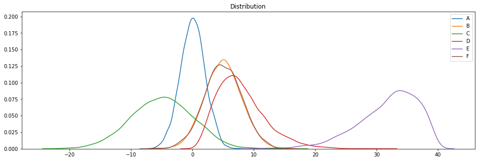
These datasets are based on Gaussian (A, B, C and F), X2 (D) and beta (E) distributions ( thanks to the Numpy np.random functions ).

This code is reusable on purpose so that you can vary the datasets and test the techniques presented.

The techniques

Basically Scikit-Learn ( sklearn.preprocessing ) provides several scaling techniques, we’ll go over 4 of them:

• MaxAbsScaler
• MinMaxScaler
• StandardScaler
• RobustScaler

MaxAbsScaler ()

This scaling technique is useful when the distribution of values ​​is sparse and you have a lot of outiers. Indeed the other techniques will tend to erase the impact of the outliers which is sometimes annoying. It is therefore interesting:

• Because robust to very small standard deviations
• It preserves null entries on a scattered data distribution

scaler = MaxAbsScaler()
keepCols = ['A', 'B', 'C']
scaled_df = scaler.fit_transform(df[keepCols])
scaled_df = pd.DataFrame(scaled_df, columns=keepCols)
plotGraph(df[keepCols], scaled_df)

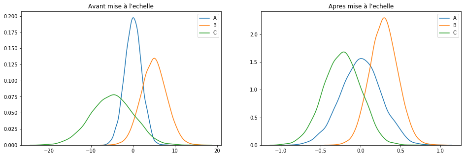
Pour résumer : cette technique se contente de rassembler les valeurs sur une plage de [-1, 1].

To summarize: this technique just collects the values ​​over a range of [-1, 1].

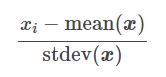
MinMaxScaler ()

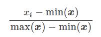
This technique transforms the characteristics (xi) by adapting each one over a given range (by default [-1 .. 1]). It is possible to change this range via the parameters feature_range = (min, max). To keep it simple, here is the transformation formula for each characteristic:

Let’s see it at work:

scaler = MinMaxScaler()
keepCols = ['A', 'B', 'C']
scaled_df = scaler.fit_transform(df[keepCols])
scaled_df = pd.DataFrame(scaled_df, columns=keepCols)
plotGraph(df[keepCols], scaled_df)

If this technique is probably the best known, it works especially well for cases where the distribution is not Gaussian or when the [itg-glossary href = ”http://www.datacorner.fr/glossary/ecart-type / “Glossary-id =” 15640 ″] Standard Deviation [/ itg-glossary] is low. However and unlike the MaxAbsScaler () technique, MinMaxScaler () is sensitive to outliers. In this case, we quickly switch to another technique: RobustScaler ().

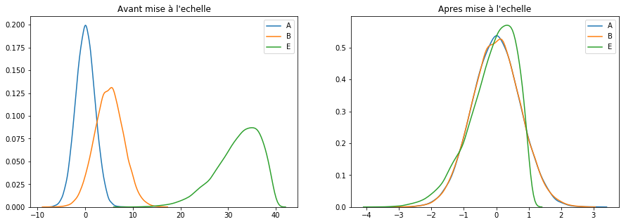
RobustScaler ()

The RobustScaler () technique uses the same scaling principle as MinMaxScaler (). However, it uses the interquartile range instead of the min-max, which makes it more reliable with respect to outliers. Here is the formula for reworking the characteristics:

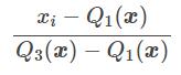
Q1 (x): 1st quantile / 25%

Q3 (x): 3rd quantile / 75%

Let’s see it at work:

scaler = RobustScaler()
keepCols = ['A', 'B', 'E']
scaled_df = scaler.fit_transform(df[keepCols])
scaled_df = pd.DataFrame(scaled_df, columns=keepCols)
plotGraph(df[keepCols], scaled_df)

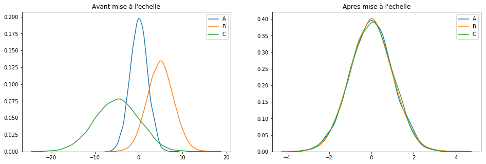
StandardScaler ()

We will finish our little tour (not exhaustive) of scaling techniques with probably the least risky: StandardScaler ().

This technique assumes that data is normally distributed. The function will recalculate each characteristic (Cf. formula below) so that the data is centered around 0 and with a [itg-glossary href = “http://www.datacorner.fr/glossary/ecart-type/” glossary-id = “15640 ″] Standard deviation [/ itg-glossary] of 1.

stdev (x): “Standard Deviation” in English means [itg-glossary href = “http://www.datacorner.fr/glossary/ecart-type/” glossary-id = “15640 ″] Standard Deviation [/ itg -glossary]

Let’s see it at work:

scaler = StandardScaler()
keepCols = ['A', 'B', 'C']
scaled_df = scaler.fit_transform(df[keepCols])
scaled_df = pd.DataFrame(scaled_df, columns=keepCols)
plotGraph(df[keepCols], scaled_df)

Conclusion

Let’s simply summarize the Feature Scaling techniques that we have just encountered:

• MaxAbsScaler: to be used when the data is not in normal distribution. Takes into account outliers.
• MinMaxScaler: calibrates the data over a range of values.
• StandardScaler: recalibrates the data for normal distributions.
• RobustScaler: same as Min-Max but uses interquartile range instead of Min and Max values.